Chapter 1: Set Theory

Mathematics is fundamentally about studying patterns, structures, quantities, and logical reasoning. In this context, set theory is a part of the foundational language of mathematics, providing an important framework for clearly describing and discussing collections of objects. Understanding sets and their notation is crucial as they form the basis for more complex mathematical structures and reasoning.

Set Basics

Definition of a Set

Definition: A Set

A diagram illustrating a set as a collection of distinct elements ( $x$ , $y$ , $z$ ) within a labeled region, along with a single element ( $w$ ) not in the set.

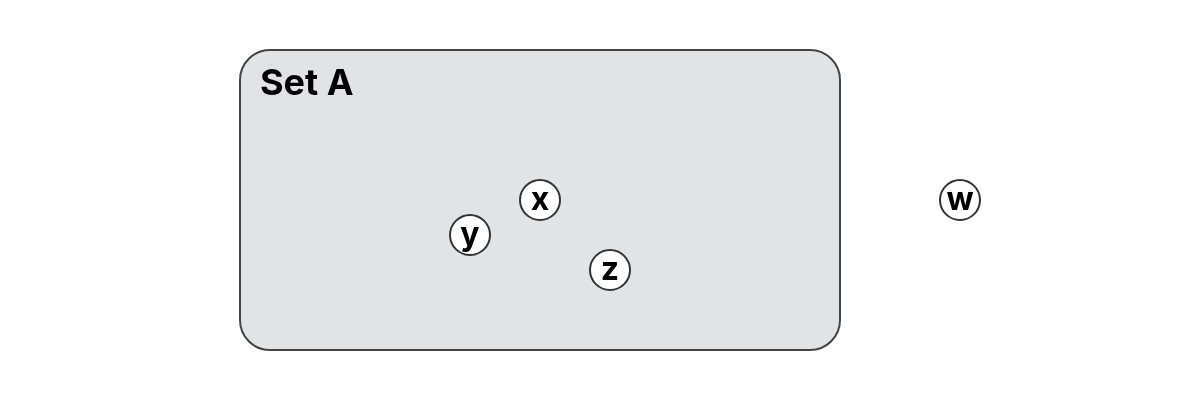
A set is a well-defined collection of distinct objects, called elements.

Notation: Sets are typically written using curly braces ${}$ and denoted by capital letters from the Latin alphabet, such as $A = {x, y, z}$ .
Well-defined: The objects inside a set, i.e., its elements, must be well-defined, meaning it is always clear whether something belongs to the set or not.
Distinct Elements: A set contains only distinct elements; no duplicates are allowed.
Order Independence: The order of elements in a set does not matter. For example, ${x, y, z}$ and ${z, x, y}$ represent the same set.

The elements $x$ , $y$ , and $z$ are placeholders and can represent anything — numbers, symbols, objects, or even abstract concepts — as long as they are clearly identifiable.

To better solidify the concept of a set, we now present a few illustrative examples.

Example: A Set

Consider the set of vowels in the English alphabet:

$A = {a, e, i, o, u}$

This set clearly lists all the vowels, and it is easy to determine whether a given letter is a vowel or not.

Example: Well-defined

For a set to be meaningful, it must be well-defined. This means it must be clear whether any given object is an element of the set or not. For example, the set of vowels in the word "radio" is well-defined and can be written as:

$A = {a, i, o}$

Similarly, the "set of all days last year with temperatures below $0^{\circ}$ C" is well-defined because it is based on objective, measurable data. However, the "set of all cold days last year" is not well-defined because the term "cold" is subjective and can vary from person to person.

Example: Distinct Elements

The set of vowels in the English alphabet is:

$A = {a, e, i, o, u}$

Note that the following is not a valid set because it contains duplicate entries:

$A = {a, a, e, i, o, u}$

In sets, each element must be distinct, so duplicates are not allowed.

Example: Order Independence

Consider two sets containing the vowels in the English alphabet:

$A = {a, e, i, o, u} and B = {u, o, i, e, a}$

These two sets are identical because they contain the same elements, regardless of the order in which the elements are listed. Thus, we can write:

$A = B$

This example illustrates the concept of order independence in sets, where the arrangement of elements does not define the uniqueness of a set.

Definition: The Empty Set

The empty set is the unique set that contains no elements. It is denoted by $\emptyset$ or simply ${}$ .

Even though it has no elements, it plays a key role in set theory, similar to how $0$ plays a key role in arithmetic.

Representing Sets

Sets can be described using various notations, each suited to different contexts. Choosing the appropriate notation depends on the nature of the set (finite vs. infinite, discrete vs. continuous) and the intended level of clarity of communication. Below, we discuss the most common methods of representing sets, along with their advantages and typical use cases.

Verbal Description

A verbal description uses ordinary language to define a set by explaining its elements or properties. This approach is particularly useful for introducing abstract or unfamiliar sets in an intuitive way or for providing context before formalizing the set with mathematical notation.

Examples: Describing Sets Verbally

"The set of vowels in the English alphabet."
"The set of whole numbers."
"The set of whole numbers strictly smaller than 6."

Roster Form

Roster form explicitly lists all elements of a set enclosed in curly braces ${}$ . This notation is particularly useful for finite sets or infinite sets with clear, recognizable patterns.

Examples: Describing Sets in Roster Form

The set of vowels in the English alphabet: ${a, e, i, o, u}$
The set of whole numbers: ${0, 1, 2, 3, 4, \dots}$
The set of whole numbers strictly smaller than 6: ${0, 1, 2, 3, 4, 5}$

Note: The ellipsis ( $\dots$ ) indicates that the pattern continues indefinitely.

Set-Builder Notation

Set-builder notation provides a precise and compact way to define a set by specifying the properties that its elements must satisfy. The notation takes one of two equivalent forms:

${x ∣ condition on x} or {x : condition on x}$

Both forms are read as "the set of all $x$ such that the given condition holds".

Here, the symbol $x$ represents a generic element of the set, i.e., it does not refer to any particular element but serves as a placeholder for all possible elements that satisfy the condition. The vertical bar ( $∣$ ) or colon ( $:$ ) functions as a divider between the variable and the rule that determines which elements belong to the set.

For example, the condition might express a numerical restriction such as $x > 0$ (meaning $x$ is strictly greater than zero), a combined relationship like $0 < x < 10$ (meaning $x$ lies strictly between zero and ten), or a membership rule such as $x \in A$ (meaning $x$ is an element of the set $A$ ). In each case, the notation highlights the defining property rather than listing individual elements.

Because of this, set-builder notation is preferred when working with infinite sets, continuous intervals, or sets defined by more complex conditions.

Examples: Describing Sets Using Set-Builder Notation

The set of vowels in the English alphabet: $A = {x ∣ x is a vowel in the English alphabet}$
The set of whole numbers: $B = {x ∣ x is a whole number}$
The set of whole numbers strictly smaller than 6: $C = {x ∣ x is a whole number and x < 6}$

Interval Notation

Certain sets appear so frequently in mathematics that they are assigned dedicated symbols. One of the most fundamental is the set of real numbers, denoted by $R$ . This set, also often just called the "reals", includes virtually any number we can think of, such as $2$ , $3$ , $44993$ , $\frac{1}{2}$ , $\frac{2}{3}$ $π$ , $e$ , and $2$ .

Geometrically, $R$ can be visualized as an infinite line, where each point corresponds to a real number. Intervals are contiguous segments of this line, representing subsets of $R$ .

An illustration of the real number line extending from $- \infty$ to $\infty$ , with the origin $0$ at the center. Positive numbers lie to the right of the origin, while negative numbers lie to the left. Every point on the line corresponds to a unique number.

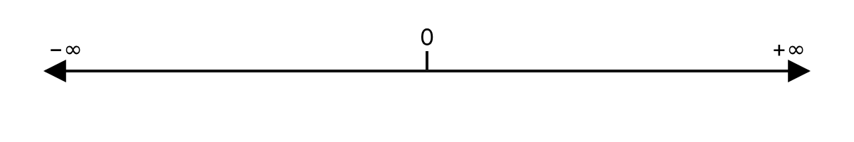
To describe intervals concisely, we use interval notation, which employs brackets $[]$ to indicate inclusive bounds and/or parentheses $()$ to indicate exclusive bounds.

Below is a summary of how interval notation corresponds to sets of real numbers together with their corresponding set-builder notation.

Set	Interval Notation	Set-Builder Notation
All real numbers	$(- \infty, \infty)$	${x ∣ x \in R}$
Open interval	$(a, b)$	${x ∣ a < x < b}$
Closed interval	$[a, b]$	${x ∣ a \leq x \leq b}$
Infinite to the right	$[a, \infty)$	${x ∣ x \geq a}$
Infinite to the right	$(a, \infty)$	${x ∣ x > a}$
Infinite to the left	$(- \infty, b]$	${x ∣ x \leq b}$
Infinite to the left	$(- \infty, b)$	${x ∣ x < b}$
Half-open (left open)	$(a, b]$	${x ∣ a < x \leq b}$
Half-open (right open)	$[a, b)$	${x ∣ a \leq x < b}$

Understanding how elements relate to sets is fundamental — not only when defining a single set, but also when comparing and working with multiple sets. In the next section, we explore these relationships in more detail and introduce their formal notation.

Examples: Describing Sets Using Intervals

Real numbers strictly between $0$ and $1$ : $(0, 1) = {x \in R ∣ 0 < x < 1}$
Real numbers between $2$ and $5$ , including both endpoints: $[2, 5] = {x \in R ∣ 2 \leq x \leq 5}$
Real numbers greater than $3$ : $(3, \infty) = {x \in R ∣ x > 3}$
Real numbers less than or equal to $0$ : $(- \infty, 0] = {x \in R ∣ x \leq 0}$

Set Membership

Set membership describes the fundamental relationship between elements and a set. This relationship is crucial for defining and understanding the contents of sets.

Definition: Set Membership

A diagram showing a set $A$ containing an element $x$ but not an element $y$ , illustrating the membership relation.

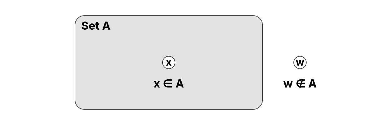
Let $x$ be an element and $A$ a set. We say that $x$ is an element (or member) of $A$ , written $x \in A$ , if and only if $x$ belongs to the collection of elements that make up $A$ . If an element $w$ is not in $A$ , we write $w \in / A$ .

Examples: Set Membership

The following examples illustrate how we use the symbols $\in$ (is an element of) and $\in /$ (is not an element of) to describe whether a value belongs to a particular set.

The element $3$ belongs to the set because it appears among its members: $3 \in {1, 2, 3, 4, 5}$
The element $6$ does not belong to the set because it is not included among its elements: $6 \in / {1, 2, 3, 4, 5}$
The number $π$ is a real number, so it belongs to the set of all real numbers: $π \in R$
In this case, the elements of the outer set are themselves sets, so ${1}$ is one of its members: ${1} \in {{1}, {2}, {3}}$
The number $1$ alone is not a member, because the set only contains sets as elements: $1 \in / {{1}, {2}, {3}}$
The fraction $\frac{7}{4}$ (equal to $1.75$ ) is in the interval because $1 \leq \frac{7}{4} < 2$ : $\frac{7}{4} \in [1, 2)$
The number $- 5$ is not in this interval because it is not positive: $- 5 \in / (0, \infty)$

This binary relationship, where each element either belongs to a set or does not, precisely defines a set’s contents and forms the basis for defining equality and more advanced set relations.

Definition: Equality of Sets

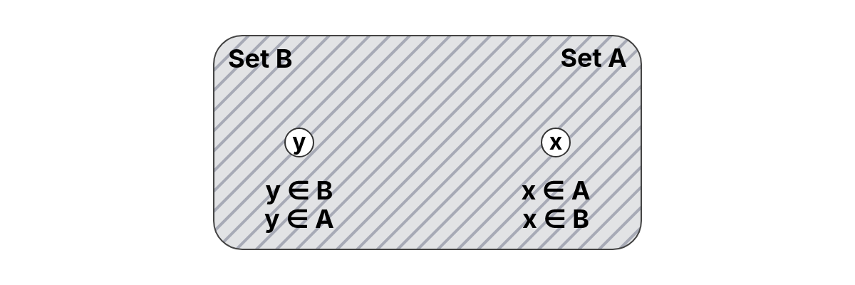
Two sets $A$ and $B$ are equal, denoted $A = B$ , if they contain exactly the same elements. This means every element of $A$ is in $B$ , and every element of $B$ is in $A$ . More formally, in predicate logic, we can write this as:

$A = B ⟺ \forall x (x \in A ⟺ x \in B)$

Or in plain words: Two sets $A$ and $B$ are equal if and only if every element $x$ belongs to $A$ exactly when it belongs to $B$ .

Cardinality

Definition: Cardinality

The cardinality of a set $A$ , written $∣ A ∣$ , indicates the number of elements in $A$ . In other words, the cardinality is the size of $A$ .

Examples: Cardinality

If $A = {a, e, i, o, u}$ , then $∣ A ∣ = 5$ . This means that $A$ is a finite set and has five distinct elements.
If $B = {1, 2, 3, 4, 5, 6}$ , then $∣ B ∣ = 6$ . This means that $B$ is a finite set and has six distinct elements.
If $C = {1, 2, 3, \dots}$ , then $∣ C ∣ = ℵ_{0}$ (aleph-null, the cardinality of any countably infinite set). This means that $C$ is countably infinite, i.e., its elements can be listed one by one in an endless sequence (first 1, then 2, then 3, and so on).
If $D = R$ , then $∣ D ∣ = c$ (the cardinality of the continuum). The set of real numbers is uncountably infinite, it is so large that it is impossible to list all elements in any sequence; between any two real numbers, there are infinitely many others.
If $E = \emptyset$ , then $∣ E ∣ = 0$ . The empty set contains no elements, so its cardinality is zero.

Equivalence of Sets

Definition: Equivalence of Sets

Two sets $A$ and $B$ are said to be equivalent, often written $A \sim B$ , if they have the same number of elements.

Formally, $A$ and $B$ are equivalent if there exists a one-to-one correspondence (a bijection) between their elements, i.e., each element of $A$ can be paired with exactly one element of $B$ , and every element of $B$ is matched with exactly one element of $A$ .

In terms of size, this means their cardinalities are equal: $∣ A ∣ = ∣ B ∣$

Examples: Equivalence of Sets

Consider the two sets of numbers: $A = {1, 2, 3}, B = {3, 2, 1} .$

These sets are equal ( $A = B$ ) because they contain exactly the same elements.

Now consider:

$C = {a, b, c}, D = {x, y, z} .$

These sets are not equal, since their contents differ, but they are equivalent ( $C \sim D$ ) because each element of $C$ can be matched with one element of $D$ .

Note: Equivalence in Other Areas of Mathematics

In most cases, we care about equality when we want to check whether two things are exactly the same. But sometimes we only care whether two things share a certain property, for example, having the same size, and that is where equivalence becomes useful.

The same idea appears in many areas of mathematics. Some simple examples are:

Two fractions such as $\frac{1}{2}$ and $\frac{2}{4}$ are equivalent because they represent the same value. Evaluating both gives $0.5$ , but the fractions themselves are written differently.
Two equations like $x + 3 = 5$ and $x = 2$ are equivalent because they have the same solution. The value $x = 2$ satisfies both equations, even though their forms differ.
Two angles are equivalent if they have the same measure, even if they open in different directions.

Two angles with equal measure are equivalent, even if they face different directions.

In geometry, shapes that are the same in size and form, though placed differently, are also considered equivalent through congruence.

Congruent shapes are equivalent because they have the same size and form.

Subsets & Proper Subsets

Subsets and proper subsets describe the relationship between sets in terms of their elements.

Definition: Subset

Diagram illustrating the subset relationship $A \subseteq B$ , where every element of $A$ is also an element of $B$ (including the case $A = B$ ).

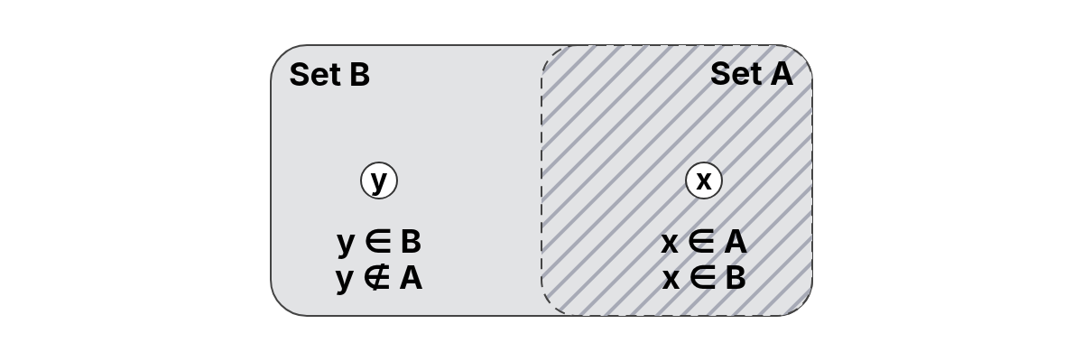
Let $A$ and $B$ be sets. We say that $A$ is a subset of $B$ if and only if every element of $A$ is an element of $B$ . We write $A \subseteq B$ to denote the fact that $A$ is a subset of $B$ .

Examples: Subset

Let $S = {3, 5, 8}$ and $T = {5, 3, 8}$ . Since both sets contain the same elements, we have that: $S \subseteq T and T \subseteq S$ Therefore, $S$ and $T$ are equal sets, and each is a subset of the other.
Let $S = \emptyset$ and $T = {5, 3, 8}$ . The empty set contains no elements, so it is a subset of every set: $S \subseteq T$
Let $S = {red, blue}$ and $T = {red, blue, green}$ . Every element of $S$ is in $T$ , so: $S \subseteq T$ Since $T$ has more elements, $S$ is also a proper subset, but we can first identify it as a subset.

Definition: Proper Subset

Diagram illustrating the proper subset relationship $A \subset B$ , where $A$ is contained within $B$ but $A \neq = B$ .

If $A$ is a subset of $B$ , but $A$ is not equal to $B$ ( $A \neq = B$ , meaning $A$ contains fewer elements than $B$ ), then $A$ is called a proper subset of $B$ , which we denote by $A \subset B$ .

If a subset contains all the elements of the original set, it is still considered a subset, but not a proper one.

Examples: Proper Subsets

Let $S = {red, blue}$ and $T = {red, blue, green}$ . Every element of $S$ is in $T$ , but $T$ has one additional element. Therefore: $S \subset T$ That is, $S$ is a proper subset of $T$ .
Similarly, if we let $S = {3, 5, 8}$ and $T = {5, 8, 3, 2, 6}$ , Then all elements of $S$ are contained in $T$ , but $T$ has additional elements ( $2$ and $6$ ). Hence: $S \subset T$ That is, again, $S$ is a proper subset of $T$ .

These examples show that a proper subset is always strictly smaller, that is, a proper subset includes some, but not all, of the elements of the larger set.

The Universe and Set Complement

The universe and set complement relate to what is not contained in a given set. Before exploring complements, we must first understand the universe that defines the context for all sets.

Definition: The Universe

A diagram showing the universe $U$ as a large rectangular region containing all relevant elements, with a set $A$ represented as a subset inside it.

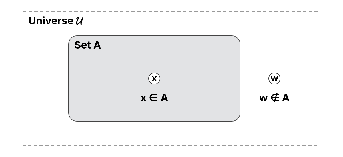
The universe, often denoted as $U$ , refers to a set that contains all the objects or elements relevant to a particular discussion or problem. It serves as the context within which all other sets are defined and interpreted.

Examples: The Universe

Let the universe be the set of all lowercase English letters: $U = {a, b, c, \dots, z} .$ Then we can define:
- $A = {x ∣ x is a vowel}$ , the set of vowels.
- $B = {x ∣ x is a consonant}$ , the set of consonants.
Here, $U$ provides a clear context: $A$ and $B$ together cover all letters in the alphabet.
Let the universe be the set of all real numbers: $U = R .$ Then we can define:
- $A = (0, 1)$ . The set of all real numbers strictly between $0$ and $1$ .
- $B = [2, 5]$ . The set of all real numbers between 2 and 5, including the endpoints.
- $C = (3, \infty)$ . The set of all real numbers greater than 3.
In this case, $U$ defines the entire number line, and each of these sets represents a subset of it.

Definition: Set Difference

Diagram showing two overlapping sets $A$ and $B$ , with $A ∖ B$ highlighted to indicate elements in $A$ that are not in $B$ .

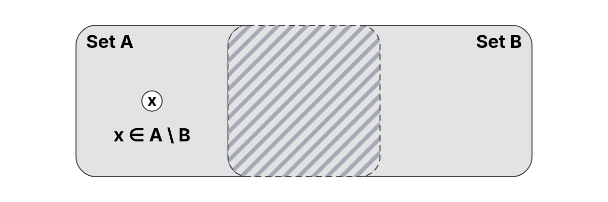
The set difference of two sets $A$ and $B$ , denoted as $A ∖ B$ , is the set of all elements that are in $A$ but not in $B$ .

$A ∖ B = {x \in A ∣ x \in / B}$

In other words, it removes from $A$ all elements that also belong to $B$ .

Examples: Set Difference

Let $A = {a, e, i, o, u}$ and $B = {a, b, c, i}$ . Then: $A ∖ B = {e, o, u} .$ These are the vowels that are not in the set $B$ .
Let $A = {1, 2, 3}$ and $B = {2, 4}$ . The elements in $A$ that are not in $B$ are: $A ∖ B = {1, 3} .$
Let $A = {apple, banana, pear}$ and $B = {pear, peach}$ . The fruits in $A$ that are not in $B$ are: $A ∖ B = {apple, banana} .$
Let $A = {1, 2}$ and $B = {1, 2}$ . Since $A$ and $B$ contain the same elements, we have that: $A ∖ B = \emptyset.$ That is, the difference is the empty set because there is nothing in $A$ that is not in $B$ .
Let $A = [0, 1]$ and $B = (0, 1)$ . Then: $A ∖ B = {0, 1} .$ The difference consists of the endpoints of the closed interval $[0, 1]$ that are not part of the open interval $(0, 1)$ .

These examples show that the set difference identifies what belongs only to the first set and not to the second.

Now that we understand how to subtract one set from another using set difference, we can define the complement of a set as a special case, subtracting from the universe.

Definition: Set Complement

Diagram illustrating the complement $A^{'}$ of a set $A$ within the universe $U$ , highlighting all elements in $U$ that are not in $A$ .

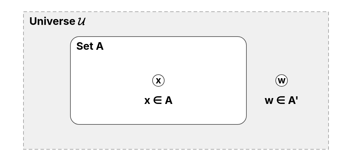
The complement of a set $A$ , denoted as $A^{'}$ , consists of all elements in the universe $U$ that are not in $A$ . In other words:

$A^{'} = U ∖ A$

The complement provides a way to discuss what is not included in a set within the context of a given universe.

Examples: Set Complement

Let $U = {1, 2, 3, 4, 5}$ and $A = {1, 2, 3}$ . The complement of $A$ is: $A^{'} = U ∖ A = {4, 5}$ Here, $A^{'}$ contains the elements of $U$ that are not in $A$ .
Let $A = {a, e, i, o, u}$ be the set of vowels in the English alphabet. If the universe $U$ is the set of all lowercase letters, then the complement $A^{'}$ is: $A^{'} = U ∖ A = all consonants in the English alphabet$ Here, the complement is expressed verbally to save space, but we could list all consonants explicitly if desired.
Let $U$ be a standard deck of playing cards, and let $A$ be the set of all spades. The complement $A^{'}$ is: $A^{'} = U ∖ A = all hearts, diamonds, and clubs.$ In this context, $A^{'}$ represents every card that is not a spade.
Let $U = R$ and $A = {x \in R ∣ x > 10}$ . The complement of $A$ is: $A^{'} = {x \in R ∣ x \leq 10}$ This means $A^{'}$ contains all real numbers less than or equal to 10.

These examples illustrate how the complement operation identifies everything outside a given set, relative to a specified universe $U$ .

Special Number Sets

As mentioned earlier, certain sets of numbers frequently appear and are often represented by special symbols. These sets range from the most basic counting numbers to the broadest set of real numbers.

Below is a summary of some of the fundamental number sets you will encounter, along with their common notations, definitions, and examples.

Fundamental Number Sets

Symbol	Name	Definition / Description
$N$	Natural numbers	${1, 2, 3, \dots}$ The counting numbers.
$N_{0}$	Natural numbers with zero	${0, 1, 2, 3, \dots}$ The natural numbers including $0$ .
$Z$	Integers	${\dots, - 2, - 1, 0, 1, 2, \dots}$ All whole numbers, both positive and negative.
$Q$	Rational numbers	${\frac{a}{b} ∣ a, b \in Z, b \neq = 0}$ The numbers that can be written as fractions.
$I$	Irrational numbers	${x \in R ∣ x \in / Q}$ The real numbers that cannot be written as fractions (e.g., $π$ , $2$ , $e$ ).
$R$	Real numbers	All numbers on the continuous number line. Includes both $Q$ and $I$ .
$C$	Complex numbers	${a + bi ∣ a, b \in R, i^{2} = - 1}$ Numbers with a real part $a$ and an imaginary part $b$ . Includes all real numbers as a subset.

These number sets are not isolated; rather, they form a natural hierarchy where smaller sets are contained within larger ones. The diagram below shows how these sets nest inside one another, for example, all natural numbers are integers, all integers are rational numbers, and all rational numbers are real numbers.

Although irrational numbers are not shown explicitly, they form the part of the real numbers that lies outside the rationals.

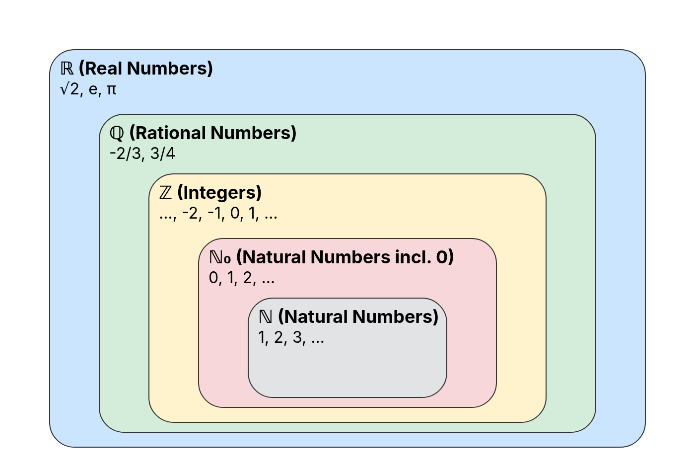
Diagram illustrating the nested hierarchy of fundamental number sets, with examples of elements in each set.

The hierarchy can also be expressed symbolically as:

$N \subset N_{0} \subset Z \subset Q \subset R \subset C$

Understanding this hierarchy helps clarify how different number systems extend one another, expanding the kinds of quantities we can represent and reason about.

Additional Set Operations

A few other foundational set operations are commonly used in mathematics and thus data science. While we will not cover these in detail in this course, the table below provides a brief overview. You will most likely encounter and work with these operations throughout your data science degree.

Symbol	Operation	Description
$A \cap B$	Intersection of $A$ and $B$	The set of all elements that are in both $A$ and $B$
$A \cup B$	Union of $A$ and $B$	The set of all elements that are in $A$ , in $B$ , or in both
$A \times B$	Cartesian product of $A$ and $B$	The set of all ordered pairs $(a, b)$ where $a \in A$ and $b \in B$
$P (A)$	The power set	The set of all subsets of $A$ , including the empty set ( $\emptyset$ ) and $A$ itself

Chapter Exercises

Exercise Set: 1

Write the following sets in roster form (if possible). If it is not possible, explain why.

The set of first five positive and even whole numbers.
The real numbers in the interval $(2, 3)$
The set of whole numbers less than 6.
The set of whole numbers that are considered very small.
The set of letters in the word "banana".
The set of even numbers that are typically interesting.
The real numbers in the interval $[2, 2]$

Use set-builder notation to describe the following sets:

${1, 2, 3, 4, 5, 6, 7}$
${1, 10, 100, 1000, 10000}$
${1, \frac{1}{2}, \frac{1}{3}, \frac{1}{4}, \frac{1}{5}, \dots}$
$[7, 7]$ , $(7, 7)$ , $(7, 7]$ and $[7, 7)$

Use interval notion to describe the following sets:

The set of all real numbers between 2 and 5, including both endpoints.
The set of all real numbers strictly greater than $- 1$ .
The set of all real numbers less than or equal to $4$ .
The set of all real numbers greater than $0$ and less than or equal to $10$ .
The empty set (in terms of intervals).

Exercise Set: 2

For each pair of sets below, determine whether they are (a) equal, (b) equivalent but not equal, (c) neither equal nor equivalent.

Let $P = {1, 2, 3, 4}$ and $Q = {3, 2, 1, 4}$
Let $P = {1, 2, 3}$ and $Q = {a, b, c}$
Let $P = {{1, 2}, {1, 3}}$ and $Q = {{1, 2}, {3, 1}}$
Let $P = {}$ and $Q = {\emptyset}$
Let $P = {{1, 2}}$ and $Q = {{1, 2}, {2, 1}}$

Let $X = {0, 1, 2}$ , $Y = {1, 2}$ , and $Z = {1, 2, 3}$ . State whether each is true, false, or meaningless:

$1 \in X$
${1} \in X$
$Y \subseteq X$
$X \subseteq Z$
$\emptyset \in Z$
$\emptyset \subseteq Z$

Exercise Set: 3

List all elements of the following sets:

${x \in N_{0} ∣ x \leq 5}$
${x \in R ∣ x^{2} = 16}$
${x \in Z ∣ - 2 \leq x \leq 2}$
${x \in Z ∣ x = x + 1}$

Let $U = {1, 2, 3, 4, 5, 6, 7, 8}$ , $A = {2, 4, 6}$ , and $B = {1, 2, 3, 4}$ . Find each of the following sets:

$A ∖ B$
$B ∖ A$
$A^{'}$
$B^{'}$
$(A ∖ B) ∖ A^{'}$

Chapter 2: Algebra

This chapter revisits some fundamental algebraic rules involving fractions, exponents, polynomials, and the use of parentheses. A firm grasp of these ideas is essential, since many common mistakes in computation and symbolic manipulation arise from misunderstanding or misapplying these basic principles.

Algebraic expressions and their underlying rules appear across a wide range of mathematical contexts. Developing the ability to recognize, interpret, and manipulate such expressions is therefore a key skill—both for simplifying symbolic formulas and for solving more complex problems in later chapters.

Note

Unless otherwise specified, all constants, variables, and placeholders are assumed to belong to subsets of the real numbers (i.e., $R$ ).

In other words, when we perform standard operations such as addition, subtraction, multiplication, or division (except division by zero), the results remain within $R$ .

Basic Algebraic Properties

Before we explore more advanced algebraic concepts, it is useful to recall a few basic properties that govern addition and multiplication. These properties, i.e., the commutative, associative, and distributive laws, apply to all real numbers and allow us to manipulate expressions, regardless of how they are written or grouped.

The Commutative, Associative & Distributive Law

The commutative law states that the order of two elements does not affect the result:

$a + b = b + a and a \cdot b = b \cdot a$

The associative law states that the way elements are grouped does not affect the result:

$(a + b) + c = a + (b + c) and (a \cdot b) \cdot c = a \cdot (b \cdot c)$

The distributive law of multiplication over addition (and subtraction):

$a \cdot (b + c) = a \cdot b + a \cdot c$

This property allows us to distribute a factor across terms inside parentheses.

Example 1: Distributive Law

Consider the expression:

$- 2 \cdot (3 + 5)$

Using the distributive law, we multiply $- 2$ by each term inside the parentheses:

$- 2 \cdot 3 + (- 2) \cdot 5 = - 6 - 10 = - 16$

The result is the same as first adding the terms inside the parentheses and then multiplying:

$- 2 \cdot (8) = - 16$

This confirms that the distributive and associative properties are consistent, i.e., the order in which we group or distribute the factors does not change the result.

Example 2: Distributive Law

Consider the expression:

$- (4 - 7)$

Here, the negative sign in front of the parentheses can be interpreted as multiplying by $- 1$ :

$- (4 - 7) = (- 1) \cdot (4 - 7)$

Applying the distributive law, we multiply $- 1$ by each term inside the parentheses:

$(- 1) \cdot 4 + (- 1) \cdot (- 7) = - 4 + 7 = 3$

This shows that placing a negative sign in front of parentheses changes the sign of each term inside.

Fractions

Fractions represent parts of a whole and are especially useful when dealing with proportions, ratios, and percentages. A fraction consists of two parts:

A numerator (top number): represents how many parts we have.
A denominator (bottom number): represents how many equal parts make up the whole.

In symbolic form, a fraction is written as a ratio of two integers:

$\frac{a}{b}, where a, b \in Z, b \neq = 0$

The set of all such numbers is called the rational numbers and denoted by $Q$ , and it forms a subset of the real numbers:

$Q \subset R$

Warning: A Common Mistake When Adding Fractions

Adding fractions is not done by simply adding the numerators and denominators:

$\frac{a}{b} + \frac{c}{d} \neq = \frac{a + c}{b + d}$

For example:
$\frac{1}{3} + \frac{1}{3} = \frac{2}{3}$ but $\frac{1 + 1}{3 + 3} = \frac{2}{6} = \frac{1}{3}$ which is incorrect for addition. Always use a common denominator as explained below.

Rule: Addition of Fractions

To add or subtract fractions, the denominators must be the same. Once a common denominator is found, we can add (or subtract) the numerators and keep the denominator unchanged.

If the denominators are already the same: $\frac{a}{c} + \frac{b}{c} = \frac{a + b}{c}$

If they are different, multiply each numerator by the other fraction’s denominator to obtain a common base: $\frac{a}{c} + \frac{b}{d} = \frac{a \cdot d + b \cdot c}{c \cdot d}$

Examples: Adding and Subtracting Fractions

Evaluate the following expression (fractions with the same denominator): $\frac{2}{5} + \frac{1}{5} = \frac{2 + 1}{5} = \frac{3}{5}$
Evaluate the following expression (fractions with different denominators): $\frac{1}{2} + \frac{1}{3} = \frac{1 \cdot 3 + 1 \cdot 2}{2 \cdot 3} = \frac{3 + 2}{6} = \frac{5}{6}$
Evaluate the following expression (subtracting two fractions): $\frac{5}{6} - \frac{1}{3} = \frac{5 \cdot 3 - 1 \cdot 6}{6 \cdot 3} = \frac{15 - 6}{18} = \frac{9}{18} = \frac{1}{2}$

Rule: Multiplication of Fractions

Multiplication of fractions is straightforward: multiply the numerators together and the denominators together.

$\frac{a}{b} \cdot \frac{c}{d} = \frac{a \cdot c}{b \cdot d}$

Examples: Multiplying Fractions

Evaluate the following expression (multiply two fractions directly): $\frac{2}{3} \cdot \frac{3}{4} = \frac{2 \cdot 3}{3 \cdot 4} = \frac{6}{12} = \frac{1}{2} = 0.5$ Multiplying straight across gives $\frac{6}{12}$ , which simplifies to $\frac{1}{2}$ .
Evaluate the following expression (simplify before multiplying): $\frac{5}{6} \cdot \frac{2}{5} = \frac{5 \cdot 2}{6 \cdot 5} = \frac{10}{30} = \frac{1}{3} \approx 0.33$ Since $5$ appears in both numerator and denominator, it can be simplified before or after multiplication.
Evaluate the following expression (multiply a whole number by a fraction): $3 \cdot \frac{2}{5} = \frac{3}{1} \cdot \frac{2}{5} = \frac{3 \cdot 2}{1 \cdot 5} = \frac{6}{5} = 1.20$ Whole numbers can be treated as fractions with denominator $1$ , making the same rule apply.

Rule: Division of Fractions

To divide one fraction by another, multiply the first fraction by the reciprocal (or multiplicative inverse) of the second fraction.

$\frac{\frac{a}{b}}{\frac{c}{d}} = \frac{a}{b} \cdot \frac{d}{c} = \frac{a \cdot d}{b \cdot c}$

Examples: Dividing Fractions

Evaluate the following expression (divide one fraction by another): $\frac{\frac{3}{4}}{\frac{2}{5}} = \frac{3}{4} \cdot \frac{5}{2} = \frac{3 \cdot 5}{4 \cdot 2} = \frac{15}{8} = 1.875$ The reciprocal of $\frac{2}{5}$ is $\frac{5}{2}$ ; multiplying gives $\frac{15}{8}$ .
Evaluate the following expression (divide by a smaller fraction): $\frac{\frac{5}{6}}{\frac{1}{2}} = \frac{5}{6} \cdot \frac{2}{1} = \frac{5 \cdot 2}{6 \cdot 1} = \frac{10}{6} = \frac{5}{3} \approx 1.66$ Dividing by a smaller fraction increases the result, since $\frac{1}{2}$ fits multiple times into $\frac{5}{6}$ .
Evaluate the following expression (divide a fraction by a whole number): $\frac{\frac{7}{9}}{7} = \frac{\frac{7}{9}}{\frac{7}{1}} = \frac{7}{9} \cdot \frac{1}{7} = \frac{7 \cdot 1}{9 \cdot 7} = \frac{7}{63} = \frac{1}{9} \approx 0.11$ Note here that the whole number $7$ can be written as $\frac{7}{1}$ , and its reciprocal is $\frac{1}{7}$ .

Note

The rational numbers $Q$ are closed under addition, subtraction, multiplication, and division (except division by zero). This means performing these operations on fractions always produces another rational number.

Exponents

Exponents indicate how many times a base number is multiplied by itself. For example:

$1^{2} = 1 \cdot 1 or 4^{3} = 4 \cdot 4 \cdot 4$

In these expressions, the base ( $1$ and $4$ , respectively) tells us what to multiply, while the exponent ( $2$ and $3$ , respectively) tells us how many times to multiply it.

Exponents essentially provide a compact way to represent repeated multiplication and follow a consistent set of algebraic rules, which we go into details with below.

Rule: Power of Zero

For any nonzero base $a$ , raising it to the power of zero equals 1:

$a^{0} = 1$

The reason $a$ must be nonzero is to avoid ambiguity. Depending on how we reason about it, we can arrive at two conflicting interpretations. From one perspective, since $0^{x} = 0$ for any positive $x$ , it might seem natural to conclude that $0^{0} = 0$ . From another, because $a^{0} = 1$ for any positive $a$ , one could instead argue that $0^{0} = 1$ . These two lines of reasoning contradict each other, so $0^{0}$ is left undefined to avoid inconsistency.

Rule: Product of Powers

When multiplying powers that share the same (nonzero) base ( $a$ ), we add their exponents ( $n$ and $m$ ):

$a^{n} \cdot a^{m} = a^{n + m}$

This rule follows from the idea that each exponent represents repeated multiplication of the same base, and combining them extends that repetition into just a single product.

Examples: Product of Powers

In the following we apply the Product of Powers rule to see how it works. That is, we evaluate the following expression: $2^{4} \cdot 2^{2} = 4 + 2 = 6 factors in total (2 \cdot 2 \cdot 2 \cdot 2) \cdot (2 \cdot 2) = 2^{6} = 64$

Here, each exponent counts how many times the base 2 appears as a factor. Combining both terms gives $4 + 2 = 6$ factors of 2 in total.

Rule: Power of a Power

When raising an exponential term ( $a^{n}$ ) to another power ( $m$ ), we simply multiply the exponents:

$(a^{n})^{m} = a^{n \cdot m}$

This rule reflects that each copy of $a^{n}$ contributes $n$ factors of $a$ , and there are $m$ such copies in total, giving us $n \cdot m$ factors altogether.

Examples: Power of a Power

In the following we apply the Power of a Power rule to see how it works. That is, we evaluate the following expression:

$(5^{3})^{2} = 5^{3} \cdot 5^{3} = 3 \cdot 2 = 3 + 3 = 6 factors in total (5 \cdot 5 \cdot 5) \cdot (5 \cdot 5 \cdot 5) = 5^{3 \cdot 2} = 5^{6} = 15, 625$

Here, the inner exponent ( $3$ ) tells us there are three factors of 5 in each group, and the outer exponent ( $2$ ) tells us there are two such groups. Altogether, we get $3 \times 2 = 6$ factors of 5.

Rule: Negative Exponent

When a base ( $a$ ) is raised to a negative exponent ( $- n$ ), the result is the reciprocal of the base ( $\frac{1}{a}$ ) raised to the corresponding positive exponent ( $n$ ):

$a^{- n} = \frac{a ^{- n}}{1} = \frac{1}{a ^{n}}, a \neq = 0$

This rule essentially expresses that a negative exponent "flips" the base, moving it from the numerator to the denominator.

Examples: Negative Exponent

Let us apply the Negative Exponent rule to see how it works.

First let us evaluate an expresseion when the base is positive:

$2^{- 3} = \frac{1}{2 ^{3}} = \frac{1}{2 \cdot 2 \cdot 2} = \frac{1}{8}$

Next, we evaluate an expression when the base is negative:

$(- 5)^{- 2} = \frac{1}{( - 5 ) ^{2}} = \frac{1}{- 5 \cdot - 5} = \frac{1}{25}$

Rule: Quotient of Powers

When dividing powers that share the same base ( $a$ ), then we subtract the exponents ( $n$ and $m$ ).

This rule follows directly from the Product of Powers and Negative Exponent rules, i.e., division is simply multiplication by the reciprocal: $\frac{a ^{n}}{a ^{m}} = a^{n} \cdot \frac{1}{a ^{m}} = a^{n} \cdot a^{- m} = a^{n - m} (Use: Negtative Exponent Rule) (Use: Product Rule)$

This rules apply when $a \neq = 0$ , since division by zero is undefined.

Examples: Quotient of Powers

Let us apply the Quotient of Powers rule to see how it works directly:

$\frac{3 ^{5}}{3 ^{2}} = 3^{5 - 2} = 3^{3} = 3 \cdot 3 \cdot 3 = 27$

We can also expand the numerator and denominator to illustrate how factors cancel out:

$\frac{3 ^{5}}{3 ^{2}} = \frac{3 \cdot 3 \cdot 3 \cdot 3 \cdot 3}{3 \cdot 3} = 3 \cdot 3 \cdot 3 = 3^{5 - 2} = 3^{3} = 27$

Here, the two factors of 3 in the denominator remove two factors from the numerator, leaving $5 - 2 = 3$ factors in total.

Rule: Fractional Exponents (Roots as Powers)

Roots can be expressed as fractional exponents. In general, the $r$ -th root of $a$ can be written as follows:

$a^{\frac{1}{r}} = r a$

This allows us to apply exponent rules even when working with roots, as roots are simply another form of exponentiation.

Examples: Fractional Exponents (Roots as Powers)

Let us apply the rule by expressing roots as fractional exponents:

The square root of a number: $a = a^{\frac{1}{2}}$
The cube root of a number: $3 a = a^{\frac{1}{3}}$
The fourth root of a power: $4 a^{3} = a^{\frac{3}{4}}$

Here, the denominator of the exponent corresponds to the root, while the numerator corresponds to the power.

Rule: Product of Roots

The root of a product is equal to the product of the roots (for non-negative $a$ and $b$ ):

$(ab)^{\frac{1}{r}} = a^{\frac{1}{r}} \cdot b^{\frac{1}{r}}, a, b \geq 0$

For square roots ( $r = 2$ ), this simplifies to:

$ab = a \cdot b$

This property holds only for non-negative real numbers, since roots of negative numbers are not real (they care complex numbers).

Examples: Product of Roots

Let us apply the Product of Roots rule to simplify a root expression:

$1 2^{\frac{1}{2}} = (4 \cdot 3)^{\frac{1}{2}} = 4^{\frac{1}{2}} \cdot 3^{\frac{1}{2}} = 4 \cdot 3 = 2 \cdot 3 (Using the Product of Roots Rule) (Since a^{\frac{1}{2}} = a)$

Here, expressing $12$ as $4 \cdot 3$ allows us to separate the square root into two simpler factors,
making the simplification straightforward.

Warning:

All these exponent rules apply for any real exponent, not just integers.

However, it is generally not possible to simplify expressions such as $2^{3} \cdot 3^{5}$ when the bases are different and unrelated by a common factor.

Likewise, exponent rules do not apply to addition or subtraction, so expressions like $a^{n} + b^{m}$ cannot be simplified using these rules.

Algebraic Identities

When working with algebraic expressions, we often encounter recurring patterns that make calculations simpler. The commutative, associative, and distributive laws, together with the rules of exponents, provide the foundation for manipulating and simplifying such expressions.

In particular, by applying the distributive law repeatedly, and interpreting exponents like $(a + b)^{2}$ or $(a + b)^{3}$ as repeated multiplication, we can derive a number of useful algebraic identities. These identities, summarized in the table below, describe common patterns that occur when expanding or factoring expressions and offer compact formulas that are helpful in later algebraic work.

Table 1. Common algebraic identities derived from the distributive law.

Name	Expression	Factored Form	Expanded Form
Square of a Sum	$(a + b)^{2}$	$(a + b) (a + b)$	$a^{2} + 2 ab + b^{2}$
Square of a Difference	$(a - b)^{2}$	$(a - b) (a - b)$	$a^{2} - 2 ab + b^{2}$
Difference of Squares	$a^{2} - b^{2}$	$(a - b) (a + b)$	$a^{2} - b^{2}$

Chapter Exercises

Chapter 3: Functions

Definition & Notation

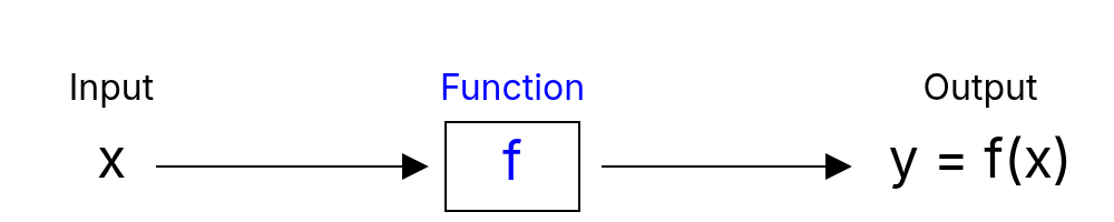
A function is a relation between two sets, where each element of the first set (called the domain) is assigned to exactly one element of the second set (called the codomain). As illustrated below, a function can be thought of as an input/output device $f$ : for any given $x$ input, the output $y = f (x)$ is uniquely determined.

*A conceptual illustration of a function as a mapping from input to output: each input $x$ is processed by a function to produce a unique output $y = f (x)$ .*

We now provide a more formal definition of a function and introduce several related concepts.

Definition: A Function

*Illustration of a function as a mapping from elements in an input set (domain) to elements in an output set (codomain).*

A function $f$ is a rule that assigns to each input $x \in A$ exactly one output $y \in B$ . This relationship is often written as:

$f : A \to B$

In particular:

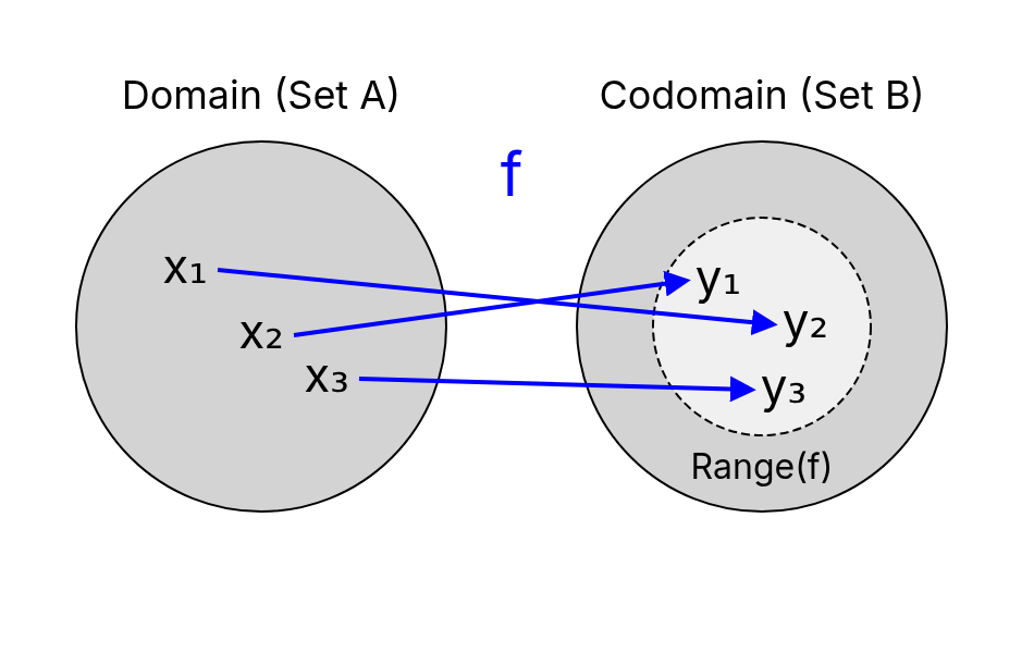
The set $A$ is called the domain of the function. It contains all possible valid inputs.
The set $B$ is called the codomain. It is the set into which all outputs are mapped.
The range (also called the image) of the function is the set of actual outputs the function produces based on its domain. It is a subset of the codomain:

$Range (f) \subseteq B$

Terminology: Independent & Dependent Variable

When we use $x$ to denote the input and $y$ to denote the output associated with $x$ , $x$ is also referred to as the independent variable and $y$ as the dependent variable, because its value "depends on $x$ ".

A function always has a domain, which is the set of all inputs for which the function is defined. If no specific domain is stated for a function given by an equation, the default is typically the set of all real numbers that yield valid (usually real) outputs.

Functions are powerful tools for describing relationships between two quantities. Many real-world scenarios can be modeled using functions, where one variable depends on another. In this context, it is also important to understand a function’s domain, codomain, and range, as these concepts help clarify what kinds of inputs are valid, what types of outputs are expected, and what outputs actually occur.

Example 1: Area of a Square

The area of a square depends on the length of its side. If the side length is $s$ , the area $A$ is given by

$A (s) = s^{2}$

Domain: $s \in [0, \infty)$ , because side lengths cannot be negative.
Codomain: $R$ , since the function produces real-number outputs (areas measured in real units).
Range: $[0, \infty)$ , because squaring any non-negative number gives a non-negative result. The smallest value occurs at $s = 0$ , where $A (0) = 0$ , and as $s$ increases, $A (s)$ grows without bound.

Example 2: Temperature Over Time

The temperature at a given time of day can be expressed as a function of time. Suppose the temperature (in °C) follows the rule

$T (t) = 10 + 8 sin (\frac{π t}{12})$

Domain: $t \in [0, 24]$ , because the model describes temperature over a single day (in hours).
Codomain: $R$ , since temperature values are real numbers.
Range: $[2, 18]$ , since the sine term $sin (\frac{π \cdot t}{12})$ varies between $- 1$ and $1$ . This means $8 sin (\cdot)$ varies between $- 8$ and $8$ , and adding $10$ shifts the range to $[2, 18]$ .

Example 3: Distance Traveled at Constant Speed

If a car travels at a constant speed of 60 km/h, the distance traveled after $t$ hours is given by

$D (t) = 60 t$

Domain: $t \in [0, \infty)$ , because time cannot be negative.
Codomain: $R$ , since distances are expressed as real numbers.
Range: $[0, \infty)$ , because multiplying a non-negative $t$ by 60 produces a non-negative result. The distance is $D (0) = 0$ at the start, and increases without bound as time increases.

Note: Choosing the Codomain

The codomain defines the set of values a function is declared to produce, while the range consists of the values that actually occur.

In many cases, the codomain is chosen to be the set of real numbers, $R$ , even when the outputs are only non-negative (as in Example 1). This convention keeps real-valued functions compatible with one another, i.e., it allows us to compare, combine, and apply the same rules (for example, addition, composition, or differentiation) without worrying about mismatched output sets.

In general, the codomain specifies the structure of the output space: it tells us what kind of values a function is expected to produce, while the range shows which of those values actually occur.

Representation Methods

Functions can be represented in several different ways, each offering different insights into the relationship they describe. Depending on the context, one representation may be more useful or informative than another.

To illustrate these representations, we will use a simplified example based on (synthetically generated) agriculture data. Let $f (x)$ denote the crop yield (in t/ha) as a function of fertilizer amount $x$ (in kg/ha). That is, we define:

$f (x) = yield corresponding to fertilizer amount x$

This example models a common real-world scenario where one quantity (fertilizer) depends on another (crop yield).

Tables

A table is one of the most straightforward ways to represent a function. This form is especially useful when working with data collected through observation or measurement. Essentially, a table just lists specific input values and their corresponding output values.

Fertilizer $x$ ( $kg/ha$ )	Crop Yield $f (x)$ ( $t/ha$ )
0	3.4942
1	3.5038
2	3.5133
3	3.5228
4	3.5322
$⋮$	$⋮$
197	4.1589
198	4.1559
199	4.1530
200	4.1500
201	4.1469
$⋮$	$⋮$
396	2.3319
397	2.3163
398	2.3008
399	2.2851
400	2.2694

In this table, each row shows a specific input value $x$ and the corresponding output value $f (x)$ . Tables are useful for answering discrete queries, such as: "What is the crop yield if given 200 kg/ha fertilizer?".

They can also help identify general trends in the data, which leads us to the following definitions.

Definition: Increasing on an Interval

We say that a function $f$ is increasing on an interval $I$ if for all $x_{1}, x_{2} \in I$ it holds that

$f (x_{1}) \leq f (x_{2}), when x_{1} < x_{2}$

The function $f$ is said to be strictly increasing (note the inequality) when

$f (x_{1}) < f (x_{2}), when x_{1} < x_{2}$

Definition: Decreasing on an Interval

We say that a function $f$ is decreasing on an interval $I$ if for all $x_{1}, x_{2} \in I$ it holds that

$f (x_{1}) \geq f (x_{2}), when x_{1} < x_{2}$

The function $f$ is said to be strictly decreasing (note the inequality) when

$f (x_{1}) > f (x_{2}), when x_{1} < x_{2}$

By applying these definitions and inspecting the table, we can observe that the crop yield $f (x)$ increases as the fertilizer amount $x$ increases - up to a certain point - and then decreases. However, beyond this general behavior, it is difficult to tell much more. The table alone does not reveal whether the relationship is simply linear, or follows a more complex curve. In particular, it does not clearly convey the rate at which the crop yield increases or whether this rate changes over the domain. For such insights, a graphical or algebraic representation is usually more informative.

Graphs

A visual picture of a function can be provided in the form of a graph. The graph of a function is the set of points $(x, f (x))$ plotted in a coordinate plane, where $z = f (x)$ for all $x$ in the domain of $f$ . Plotting data points from a table helps reveal the overall shape and behavior of the function, which may not be immediately apparent from a list of values alone.

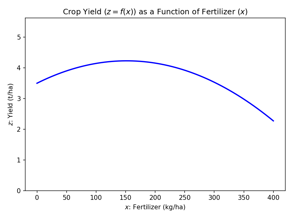
From this graph, we can observe that the function increases with fertilizer ( $x$ ), to a point, but not linearly. The curve appears to flatten and then decrease more sharply, suggesting that the relationship between fertilizer ( $x$ ) and yield ( $f (x)$ ) is non-linear, possibly polynomial.

Algebraic Formulas

Often, we want more than just individual data points, we want a general rule that allows us to compute the output for any valid input. An algebraic formula provides a compact, symbolic way to describe the relationship between inputs and outputs.

The table and graphs shown above of the crop yield have actually been generated based on the quadratic polynomial:

$f (x) = - 3.17042 \cdot 1 0^{- 5} \cdot x^{2} + 0.00961968 x + 3.49418$

This expression is not arbitrary, it was obtained from observed data using a method that fits a mathematical function to the measurements. In this case, the polynomial gives an approximation of the relationship between fertilizer amount and crop yield, smoothing out random variations while preserving the overall pattern seen in the data.

Having an algebraic representation allows us to carry out several useful analyses:

Interpolation: Estimate values between known data points.
Extrapolation: Predict behavior beyond the observed range, for instance, for very small or large fertilizer amounts ( $x$ ).
Equation solving: Find input values corresponding to specific outputs, for example solving $f (x) = 4.5$ to determine the corresponding fertilizer amount that yields 4.5 t/ha.

More broadly, models based on algebraic formulas let us describe and explore real-world phenomena: how quantities change together, where growth slows or reverses, and how one variable influences another. Such models form the foundation of mathematical analysis, offering insight into underlying behavior.

To describe these relationships effectively, we must choose a suitable type of function and fit it to the data. In this example, the coefficients of the polynomial were determined using least squares regression, a method that finds the curve that best matches the observed data. Recognizing different classes of functions, such as linear, quadratic, cubic, or exponential, helps us select appropriate models and interpret the types of behavior they represent.

Basic Classes of Functions

Functions can be grouped into different classes based on their algebraic form. Each class has its own properties, domain and range, and characteristic graph shape. In this section, we focus on common basic function classes and describe their general forms (graphical) behavior.

Before exploring specific types, it is useful to note two important features that appear frequently in graphs of functions:

Feature	Definition	Why It Matters
Intercepts	Points where the graph crosses the coordinate axes. $x$ -intercepts occur when $f (x) = 0$ , and the $y$ -intercept occurs when $x = 0$ .	Represent starting values, equilibrium states, or solutions to problems.
Turning Points	Points where the graph changes direction from increasing to decreasing, or vice versa.	Indicate local maxima or minima; used to identify peaks, troughs, or optimal conditions.
Asymptotes	Lines that the graph approaches but does not cross (or only crosses at infinity): horizontal, vertical, or oblique.	Describe long-term trends or limits in growth/behavior; mark boundaries.

Polynomial Functions

Polynomial functions are smooth, continuous curves with no sharp corners or breaks. Their general behavior depends on the degree and the leading coefficient.

Definition: Polynomial Function

*Examples of polynomial functions of different degrees, showing how the degree affects the shape and number of turning points of the graph.*

Polynomials belong to a broad class of functions that can be written in the general form:

$f (x) = a_{n} x^{n} + a_{n - 1} x^{n - 1} + \dots + a_{1} x + a_{0}$

where:

$n$ is a non-negative integer (the degree of the polynomial)
$a_{n}, a_{n - 1}, \dots, a_{0}$ are real constants
$a_{n} \neq = 0$ if $n > 0$

Key characteristics:

Graph: smooth, continuous curve.
Intercepts: Up to $n$ real $x$ -intercepts; always one $y$ -intercept at $(0, a_{0})$ .
Domain: All real numbers ( $R$ )
Range: Depends on the degree and coefficients.

Terminology: Classification of Polynomials

Polynomials are commonly classified based on two characteristics:

The number of terms
The degree of the expression

The following tables summarize these classifications with corresponding examples.

Table 1. Classification of polynomials by the number of terms.

Number of Terms	Name	Example
$1$	Monomial	$5 x^{3}$
$2$	Binomial	$3 x^{2} + 1$
$3$	Trinomial	$x^{2} - 4 x + 4$
$\geq 4$	Polynomial	$x^{4} + x^{3} - 2 x + 7$

Table 2. Classification of polynomials by degree.

Degree	Name	Example
$0$	Constant	$7$
$1$	Linear	$2 x + 3$
$2$	Quadratic	$x^{2} - 4 x + 4$
$3$	Cubic	$x^{3} - x$
$4$	Quartic	$x^{4} + 2 x^{2} + 1$
$5$	Quintic	$x^{5} - x^{3} + 1$
$n \geq 6$	$n$ th-degree polynomial	$x^{6} + \dots$

Linear Functions

A linear function is a polynomial of degree $1$ and its graph is a straight line.

Definition: Linear Function

*Graphs of two linear functions. The first shows an increasing line ( $a > 0$ ), while the second shows a decreasing function ( $a < 0$ ).*

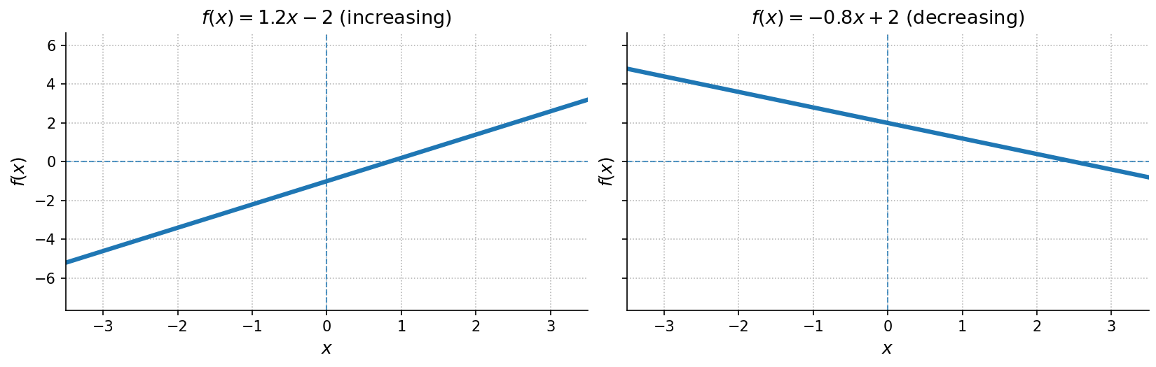
A linear function can be written in the general (slope-intercept) form:

$f (x) = a x + b$

where $a$ and $b$ are constants. If $a \neq = 0$ , it is a polynomial of degree $1$ ; if $a = 0$ , it simplifies to $f (x) = b$ , which is a constant function (a polynomial of degree 0).

Key characteristics:

Graph: A straight line with slope $a$ .
- If $a > 0$ the function is increasing
- If $a < 0$ the function is decreasing
Intercepts:
- $y$ -intercept at point $(0, b)$
- $x$ -intercept at point $(- \frac{b}{a}, 0)$
Domain: All real numbers ( $R$ )
Range: All real numbers ( $R$ )

Examples: Linear Functions

Determine which of the following functions are linear functions:

$f (x) = 3 x - 5$
$g (x) = 7$
$h (x) = 2 x^{2} + 1$

Answer: $f (x)$ is linear (degree 1), while $g (x)$ is a constant function (degree 0), and $h$ is quadratic (degree 2).

One of the defining characteristics of a line is its slope. The slope describes how a line rises or falls as we move along the $x$ -axis, i.e., in other words, it represents the rate of change in $y$ for each unit change in $x$ .

The slope measures both the steepness and the direction of a line:

If the slope is positive, the line points upward when moving from left to right
If the slope is negative, the line points downward when moving from left to right
If the slope is zero, the line is horizontal

To determine the slope numerically, we compare how much $y$ changes relative to $x$ . This comparison gives us the ratio of the change in $y$ to the change in $x$ , leading to the more formal definition below.

Definition: Slope of a Linear Function

Consider a line passing through points $(x_{1}, y_{1})$ and $(x_{2}, y_{2})$ . Let $Δ y = y_{2} - y_{1}$ and $Δ x = x_{2} - x_{1}$ denote the changes in $y$ and $x$ , respectively. The slope of the line is:

$m = \frac{y _{2} - y _{1}}{x _{2} - x _{1}} = \frac{Δ y}{Δ x}$

Now, let us explore how this definition relates to the formula of a linear function. Consider the function:

$f (x) = a x + b$

We already know that the graph of a linear function is a straight line. To find its slope, we can apply the definition above using any two points, i.e., $(x_{1}, y_{1})$ and $(x_{2}, y_{2})$ , on the line. In particular, let us evaluate the function at two convenient points:

When $x_{1} = 0$ , we have $y_{1} = f (0) = a \cdot 0 + b = b$ . This gives us the point: $(x_{1}, y_{1}) = (0, b)$
When $x_{2} = 1$ , we have $y_{2} = f (1) = a \cdot 1 + b = a + b$ . This gives us the point: $(x_{2}, y_{2}) = (1, a + b)$

Therefore, substituting the points into the formula for the slope, the slope of this line is:

$m = \frac{y _{2} - y _{1}}{x _{2} - x _{1}} = \frac{( a + b ) - b}{1 - 0} = \frac{a}{1} = a$

This shows that the coefficient $a$ in the function $f (x) = a x + b$ represents the slope of the line. Hence, every linear function of the form $f (x) = a x + b$ describes a line with slope $a$ and $y$ -intercept $b$ .

This relationship will be revisited in Chapter 8, where the concept of slope forms the basis for defining differentiation.

Quadratic Functions

A quadratic function is a polynomial of degree $2$ ; its graph is a parabola.

Definition: Quadratic Function

*Graphs of three quadratic functions. The first two parabolas open upward ( $a > 0$ ), while the last opens downward $(a < 0)$ .*

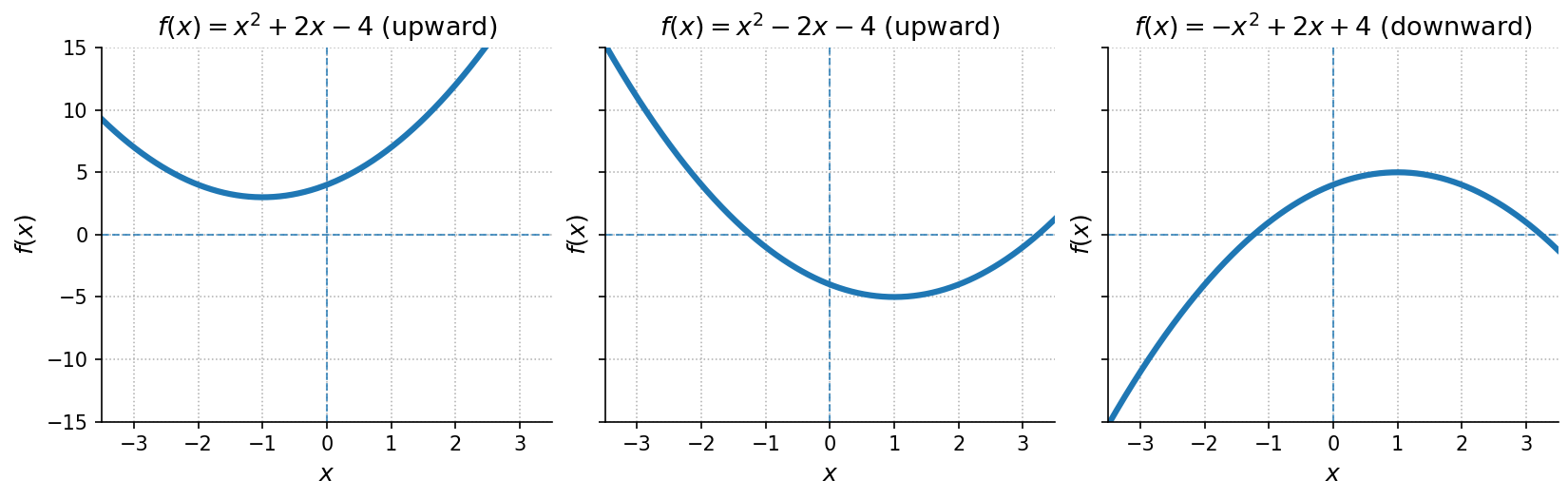
A quadratic function can be written in the general form:

$f (x) = a x^{2} + b x + c$

where $a \neq = 0$ .

Key characteristics:

Graph: A parabola.
- If $a > 0$ the parabola opens upward
- If $a < 0$ the parabola opens downward
Intercepts: Up to two $x$ -intercepts, and exactly one $y$ -intercept
Turning Point: The peak of the graph.
- If $a > 0$ it is the lowest point $(x_{m a x}, y_{m a x})$
- If $a < 0$ it is the highest point $(x_{m i n}, y_{m i n})$
Domain: All real numbers ( $R$ )
Range:
- If $a > 0$ it is $[y_{m i n}, \infty)$
- If $a < 0$ it is $(- \infty, y_{m a x}]$

Examples: Quadratic Functions

Determine which of the following functions are quadratic functions:

$f (x) = 4 x^{2} - x + 7$
$g (x) = x (x - 5)$
$h (x) = 3 x^{3} - 2 x + 1$

Answer: $f (x)$ and $g (x)$ are quadratic. $h (x)$ is cubic.

Exponential Functions

Exponential functions have a constant base raised to a variable exponent.

Definition: Exponential Function

*Examples of exponential functions. The first two illustrate exponential growth ( $b > 1$ ), while the last shows exponential decay ( $0 < b < 1$ ).*

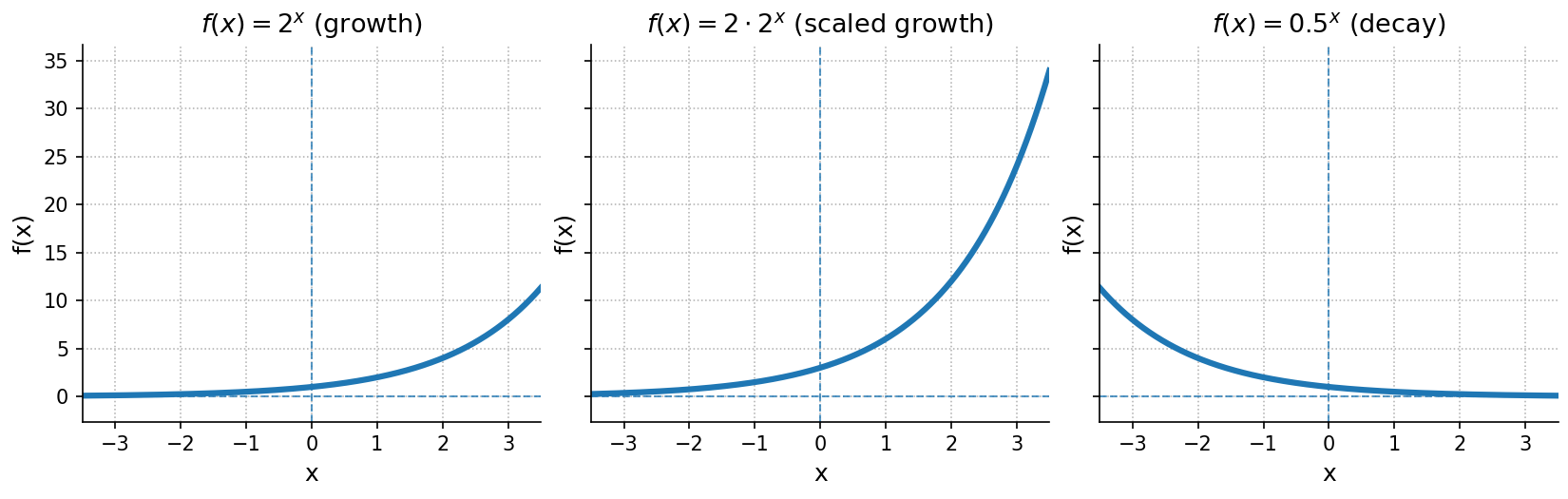
An exponential function can be written in the general form:

$f (x) = a b^{x}$

where $a \neq = 0$ , $b > 0$ , and $b \neq = 1$ .

Key characteristics:

Graph:
- If $b > 1$ the graph is increasing (growth)
- If $0 < b < 1$ the graph is decreasing (decay)
Asymptote: Horizontal at $y = 0$ .
Domain: All real numbers ( $R$ )
Range: $(0, \infty)$ if $a > 0$

Examples: Exponential Functions

Determine which of the following functions are exponential functions:

$f (x) = 2^{x}$
$g (x) = x^{2}$
$h (x) = 5 \cdot (0.5)^{x}$

Answer: $f (x)$ and $h (x)$ are exponential. Here $g (x)$ is a power function (a special case of a polynomial).

Logarithmic Function

Logarithmic functions are the inverses of exponential functions.

Definition: Logarithmic Function

*Three examples of a logarithmic functions. They are all increasing functions, scaled or using different base.*

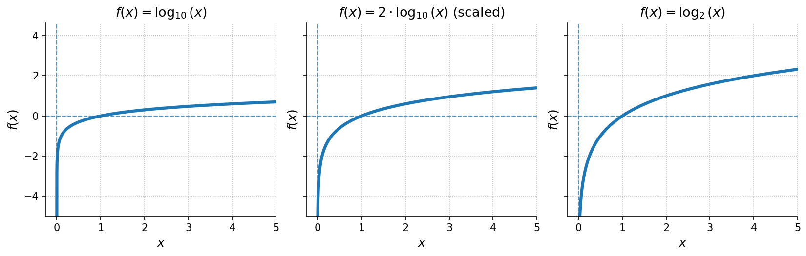
A logarithmic function can be written in the general form:

$f (x) = a \cdot lo g_{b} (x)$

where $a \neq = 0$ , $b > 0$ , and $b \neq = 1$ .

Key characteristics:

Graph:
- Passes through $(1, 0)$ if $a = 1$
- Slow, unbounded growth for large $x$
Asymptote: Vertical at $x = 0$ .
Domain: $(0, \infty)$
Range: All real numbers ( $R$ )

Examples: Logarithmic Functions

Determine which of the following functions are logarithmic functions:

$f (x) = lo g_{2} (x)$
$g (x) = ln (x)$
$h (x) = 5^{x}$

Answer: $f (x)$ and $g (x)$ are logarithmic. $h (x)$ is exponential.

Piecewise-Defined Functions

Not all functions can be described by a single formula. In some cases, different rules apply to different parts of the domain. Such functions are called piecewise-defined functions.

Definition: Piecewise Function

A piecewise-defined function is a function whose rule is given by multiple expressions, each applying to a specific interval (or subset) of the domain. Formally, it can be written as:

$f (x) = ⎩ ⎨ ⎧ f_{1} (x), f_{2} (x), ⋮ f_{n} (x), if x \in D_{1}, if x \in D_{2}, ⋮ if x \in D_{n},$

where:

Each $f_{i} (x)$ defines the function on a subset $D_{i}$ of the domain
The subsets $D_{1}, D_{2}, \dots, D_{n}$ are non-overlapping and form the entire domain of $f$
Each input $x$ belongs to exactly one of the subsets $D_{i}$ , ensuring that the function assigns one unique output for every input

Key characteristics:

Graph: May be continuous or discontinuous at the boundary points between pieces
Domain: The union of all subsets $D_{i}$
Range: The union of the output values of all pieces

Example 1: A Piecewise Function

*Graph of a piecewise-defined function with two expressions joined at $x = 2$ .*

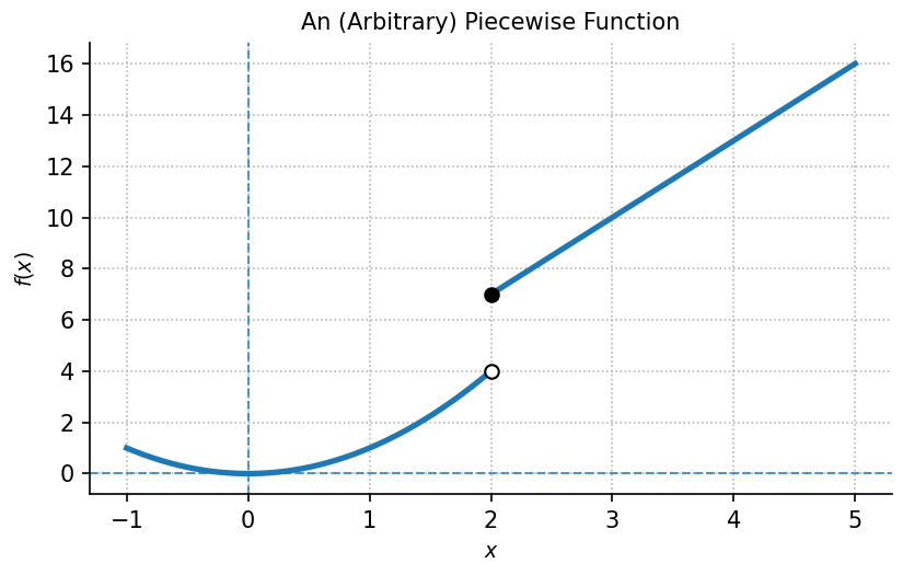
Consider the function defined by

$f (x) = {3 x + 1, x^{2}, if x \geq 2, if x < 2.$

To evaluate a piecewise function, first determine which part of the domain the input belongs to, and then apply the corresponding rule. For instance:

For $x = 5$ , since $5 \geq 2$ , use function $3 x + 1$ : $f (5) = 3 \cdot 5 + 1 = 16$
For $x = - 1$ , since $- 1 < 2$ , use function $x^{2}$ : $f (- 1) = (- 1)^{2} = 1$

Example 2: A Piecewise Function

*Graph of the absolute value function $f (x) = ∣ x ∣$ , showing a change in rule at $x = 0$ .*

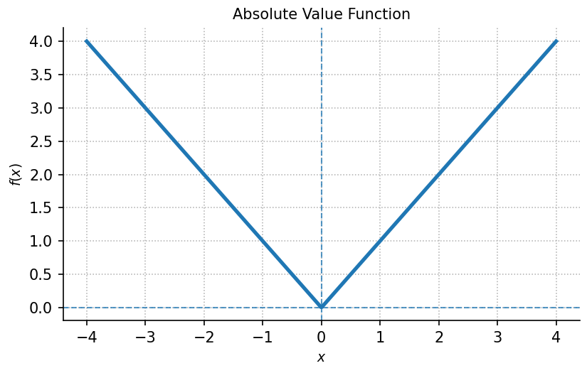
The absolute value function, denoted by $f (x) = ∣ x ∣$ , can be expressed as a piecewise-defined function:

$f (x) = {- x, - x, if x \geq 0, if x < 0.$

Here, positive inputs are unchanged, while negative inputs are reflected across the $x$ -axis, ensuring that $f (x)$ is always non-negative.

Example 3: A Piecewise Function

*Graph of the ReLU (Rectified Linear Unit) function, which outputs zero for negative inputs and increases linearly for positive inputs.*

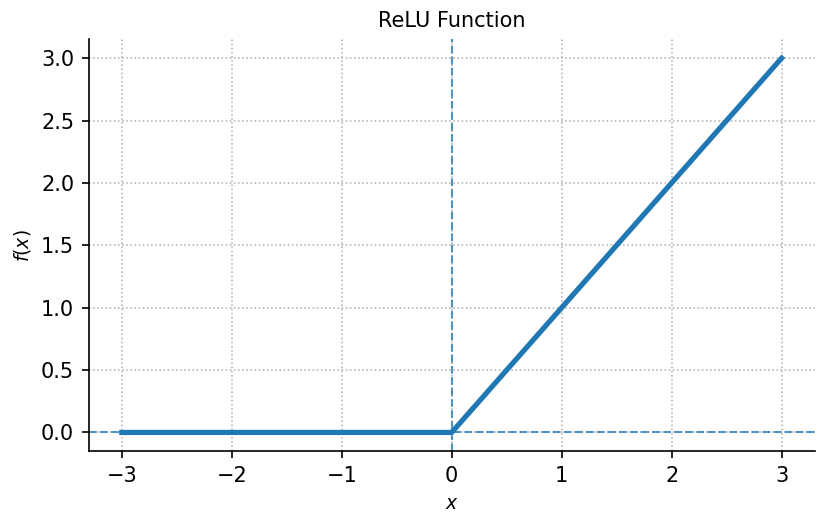
The Rectified Linear Unit (ReLU) is a commonly used activation function in neural networks. It can be expressed as a piecewise-defined function:

$f (x) = {x, 0, if x > 0, if x \leq 0.$

The ReLU function outputs the input value itself when it is positive, and zero otherwise. This simple non-linear behavior introduces nonlinearity into neural networks, which is an essential property that allows them to learn complex patterns and relationships in data.

Injective, Surjective, and Bijective Functions

Functions can also be classified based on how they relate elements of their domain to elements of their codomain. While algebraic form determines a function’s shape or formula, mapping properties determine whether the function is one-to-one, onto, or both.

Definition: Injective Function

A function $f : A \to B$ is injective (or one-to-one) if it never assigns the same output value to two different inputs. In other words, each output in $B$ comes from at most one input in $A$ .

More formally, in predicate logic, we can write:

$\forall x_{1}, x_{2} \in A, f (x_{1}) = f (x_{2}) \Rightarrow x_{1} = x_{2}$

Or in plain words: If two inputs of a function give the same output, then those inputs must be equal.

Example: Injective Function

*Left: An injective function. Right: A non-injective function.*

Let $f : R \to R$ be defined by:

$f (x) = 2 x + 3$

This function is injective because different $x$ -values always produce different $y$ -values. However, $f (x) = x^{2}$ is not injective on $R$ since $f (2) = f (- 2) = 4$ .

Definition: Surjective Function

A function $f : A \to B$ is surjective (or onto) if every element of the codomain $B$ appears as an output of the function. That means the function covers all of $B$ , i.e., its range is equal to its codomain.

More formally, in predicate logic, we can write:

$\forall y \in B, \exists x \in A such that f (x) = y$

Or in plain words: For every possible output value in the codomain, there exists at least one input value in the domain that produces it.

Example: Surjective Function

*Left: A surjective function that covers all possible $y$ -values in the codomain. Right: A non-surjective function which leaves gaps.*

Let $f : R \to R$ be defined by:

$f (x) = 2 x + 1$

For any $y \in R$ , there exists $x = \frac{y - 1}{2}$ , so $f$ is surjective. However, $f (x) = x^{2}$ from $R \to R$ is not surjective because negative $y$ -values are never reached.

Definition: Bijective Function

A function $f : A \to B$ is bijective if it is both injective and surjective. This means that each element of $A$ is mapped to a unique element of $B$ (injectivity), and every element of $B$ is the image of some element of $A$ (surjectivity).

More formally, we can write: $f is bijective ⟺ (f is injective) and (f is surjective)$

Or in plain words: A bijective function establishes a one-to-one correspondence between the sets $A$ and $B$ , so that nothing is repeated and nothing is left out.

Example: Bijective Function

*A bijective function: each element of the domain maps to exactly one unique element of the codomain.*

Let $f : R \to R$ be defined by:

$f (x) = x + 1$

The function is bijective because each input produces a unique output (injective) and every real number occurs exactly once as an output (surjective).

Combining Functions

Up to this point, we have explored the basic characteristics of individual functions. We now turn to what happens when functions are combined using standard mathematical operations to create new ones. Just as numbers can be added, subtracted, multiplied, or divided, functions can also be combined in similar ways to form new functions with related behaviors.

Example 1: Combining Functions

In machine learning, the loss function used to train a model often combines several components that measure different aspects of performance.

Suppose we define:

$f (x)$ : The prediction error
$g (x)$ : A regularization term that penalizes overly complex models

Note that $x$ may represent several model parameters, but the idea of combining functions, i.e., adding terms that capture different effects, follows the same principle as in the single-variable case.

The resulting loss function balances accuracy (how well predictions match the observed data) with simplicity (how small the model parameters are):

$L (x) = f (x) + λ \cdot g (x),$

where $λ > 0$ controls how strongly the regularization term influences the model.

Example 2: Combining Functions

In many real-world models, new relationships are created by combining existing quantities using arithmetic operations.

Suppose we define:

$f (x)$ : the temperature (in °C)
$g (x)$ : the humidity (in %)

A new function $h (x)$ can be defined to estimate a heat index (a perceived temperature) as follows:

$h (x) = f (x) + 0.1 \cdot g (x)$

Here, $h (x)$ is obtained by adding a weighted contribution from humidity to the temperature. Such combinations describe how different quantities together determine a result. In this case, both temperature and humidity contribute to the perceived heat.

Suppose $f$ and $g$ are functions defined on the same domain. The following operations define new functions as shown below:

Operation	Notation	Definition
Sum	$(f + g) (x)$	$f (x) + g (x)$
Difference	$(f - g) (x)$	$f (x) - g (x)$
Product	$(f \cdot g) (x)$	$f (x) \cdot g (x)$
Quotient	$(\frac{f}{g}) (x)$	$\frac{f ( x )}{g ( x )}, g (x) \neq = 0$

Ultimately, these operations let us construct more complex relationships from simpler ones.

Example 3: Combining Functions

In this example, we explore how subtraction and division affect the relationship between two functions. For this purpose, let

$f (x) = x - 1, and g (x) = x^{2} - 1.$

We will now find and simplify both $(g - f) (x)$ and $(\frac{g}{f}) (x)$ to see how these operations transform the expressions.

First, subtract $f (x)$ from $g (x)$ :

$(g - f) (x) = g (x) - f (x) = (x^{2} - 1) - (x - 1) = x^{2} - x = x (x - 1)$

Then, divide $g (x)$ by $f (x)$ :

$(\frac{g}{f}) (x) = \frac{g ( x )}{f ( x )} = \frac{x ^{2} - 1}{x - 1} = \frac{( x + 1 ) ( x - 1 )}{x - 1} = x + 1$

We can see that subtraction and division lead to very different results, i.e., $(g - f) (x)$ is a quadratic expression, while $\frac{g}{f}$ simplifies to a linear one.

Even though both start from the same $f$ and $g$ , the way we combine them changes the type of function we obtain.

Example 4: Combining Functions

In this example, we explore how multiplication and subtraction affect the relationship between two functions. For this purpose, let

$f (x) = x - 1, and g (x) = x^{2} - 1$

We will now find and simplify both $(f \cdot g) (x)$ and $(f - g) (x)$ to see how these operations transform the expressions.

First, multiply $f (x)$ and $g (x)$ :

$(f \cdot g) (x) = f (x) \cdot g (x) = (x - 1) (x^{2} - 1) = x^{3} - x^{2} - x + 1$

Then, subtract $g (x)$ from $f (x)$ :

$(f - g) (x) = f (x) - g (x) = (x - 1) - (x^{2} - 1) = x - x^{2}$

Again, the two resulting functions are very different, i.e., $(f \cdot g) (x)$ is cubic, while $(f - g) (x)$ is quadratic.

Function Composition

In the previous examples, we combined functions using arithmetic operations such as addition and multiplication. Now, explore a different kind of combination, i.e., function composition, where the output of one function becomes the input of another.

Function composition allows us to describe multi-step relationships between quantities that depend on one another.

In many real-world situations, one variable influences a second, which in turn affects a third. By composing functions, we can express an entire chain of dependencies as a single mathematical expression.

Example 1: Function Composition

Suppose we want to calculate how much electricity is used to cool a house on a particular day of the year. The electricity usage depends on the average indoor-outdoor temperature difference, which in turn depends on the average daily temperature outside.

Thus, we have two relationships:

$E (T)$ : Describes the electricity (in kWh) required to maintain a desired indoor temperature for a given outdoor temperature $T$ (°C)
$T (d)$ : Describes the average outdoor temperature (°C) on day $d$ of the year

For any given day $d$ , the electricity use depends on the temperature, which itself depends on the day. We can therefore evaluate $E$ at the temperature given by $T (d)$ :

$E (T (d))$

This expression represents the electricity used on day $d$ . For example, to find the electricity usage on the 10th day of the year, we would first compute $T (10)$ , the average temperature on day 10, and then use that value in function $E$ , i.e., $E (T (10))$ gives the electricity required to cool the house on the 10th day of the year.

In this case, the function describing temperature is said to be composed with the function describing electricity usage.

The relationship illustrated above can be generalized by defining a new function that represents applying one function after another. For this to be well-defined, the range of the inner function must lie within the domain of the outer function.

This brings us to the formal definition of the composition of functions.

Definition: Function Composition

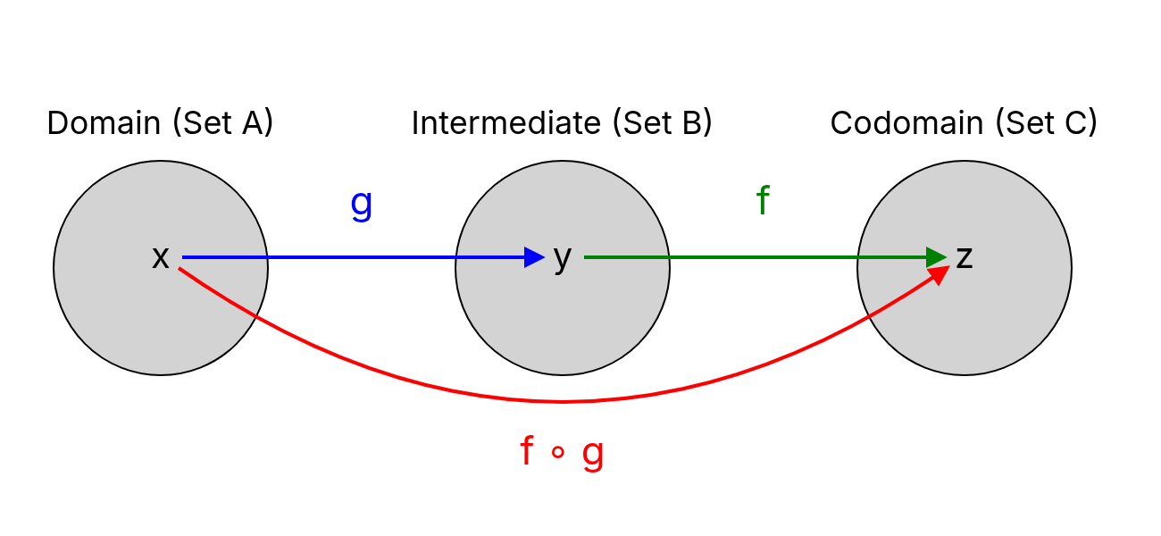
Let $f : B \to C$ and $g : A \to B$ be functions, where the codomain of $g$ (the set of its possible outputs) is contained in the domain of $f$ . The composition of $f$ and $g$ , denoted $f \circ g$ , is the function

$f \circ g : A \to C$

defined by

$(f \circ g) (x) = f (g (x)) for all x \in A .$

Warning: Misconceptions About Composition

Composition is not multiplication:

The composition of two functions is denoted by $f \circ g$ and defined as

$(f \circ g) (x) = f (g (x)) .$

In contrast, the product of two functions is denoted by $f \cdot g$ and defined as

$(f \cdot g) (x) = f (x) \cdot g (x) .$

The first applies one function inside another, while the second multiplies their outputs.
Composition is not commutative:

In general it is the case that

$f \circ g \neq = g \circ f,$

since

$f (g (x)) \neq = g (f (x))$

for most functions $f$ and $g$ . In other words, the order matters because the output of one function becomes the input of the other, and reversing that order usually produces a different intermediate value.

Example 2: Function Composition

Using the following functions, find both $f (g (x))$ and $g (f (x))$ to determine whether composition is commutative.

$f (x) = 2 x + 1, g (x) = 3 - x$

First, substitute $g (x)$ into $f (x)$ :

$f (g (x)) = 2 (3 - x) + 1 = 6 - 2 x + 1 = 7 - 2 x$

Next, substitute $f (x)$ into $g (x)$ :

$g (f (x)) = 3 - (2 x + 1) = 3 - 2 x - 1 = 2 - 2 x$

Because $f (g (x)) \neq = g (f (x))$ , we see that function composition is not commutative.

Decomposing Functions

The idea of composition naturally leads to its reverse process, i.e., decomposition. While composition builds complex relationships by applying one function after another, decomposition involves expressing a single, complicated function in terms of simpler ones:

$h (x) = (f \circ g) (x) = f (g (x))$

This approach makes functions easier to understand and, more importantly, easier to work with. It will play an important role later, particularly in Chapter 8, where recognizing how a function is composed of simpler parts becomes essential for applying the chain rule of differentiation.

Note that a single function may have more than one possible decomposition. In practice, we choose the one that makes the problem easier.

Example 1: Decomposing Functions

Express $h (x) = 5 - x^{2}$ as the composition of two simpler functions.

We are looking for functions $f$ and $g$ such that

$h (x) = (f \circ g) (x) = f (g (x))$

To identify these functions, notice that $5 - x^{2}$ appears inside the square root. This suggests the inner function produces $5 - x^{2}$ , and the outer function takes the square root of its input. Thus, we can define

$g (x) = 5 - x^{2} and f (x) = x$

We can verify our decomposition by recomposing the functions:

$(f \circ g) (x) = f (g (x)) = f (5 - x^{2}) = 5 - x^{2}$

Therefore, $h (x) = (f \circ g) (x)$ with

$g (x) = 5 - x^{2}, and f (x) = x$

Example 2: Decomposing Functions

Express $h (x) = \frac{4}{3 - 4 + x ^{2}}$ as the composition of two simpler functions.

We are looking for functions $f$ and $g$ such that

$h (x) = (f \circ g) (x) = f (g (x))$

Here, the expression $4 + x^{2}$ appears inside the denominator. We can treat that as the output of the inner function $g$ , and then let the outer function $f$ operate on that result. Thus, we can define

$g (x) = 4 + x^{2} and f (x) = \frac{4}{3 - x}$

We can verify our decomposition by recomposing the functions:

$(f \circ g) (x) = f (g (x)) = f (4 + x^{2}) = \frac{4}{3 - 4 + x ^{2}}$

Therefore, $h (x) = (f \circ g) (x)$ with

$g (x) = 4 + x^{2}, and f (x) = \frac{4}{3 - x}$

Chapter Exercises

Chapter 4: Polynomial Factorization

In the previous chapter, we introduced polynomials as a fundamental class of functions that can be written in the general form:

$f (x) = a_{n} x^{n} + a_{n - 1} x^{n - 1} + \dots + a_{1} x + a_{0}$

A polynomial consists of terms involving a variable (here, $x$ ) raised to non-negative integer powers and multiplied by constant coefficients. Formally, $n \in N_{0}$ denotes the degree of the polynomial, and $a_{n}, a_{n - 1}, \dots, a_{0} \in R$ are its coefficients, with $a_{n}$ being the leading coefficient.

In this chapter, we will learn how to manipulate and simplify polynomials in order to better understand their behavior, find their zeros, and analyze their graphs.
A key step in this process is factorization, which allows us to rewrite a polynomial as a product of simpler factors.

Before exploring general methods, recall that certain algebraic identities, introduced in Chapter 2, can be applied directly to polynomials. These identities often enable quick factorizations of specific expressions without the need for more elaborate techniques.

Example: The Square of a Difference

Suppose we want to factor the following polynomial:

$x^{2} - 4$

This expression simply matches the difference of squares identity, so we apply it directly as follow:

$x^{2} - 4 = x^{2} - 2^{2} = (x - 2) (x + 2)$

While simple cases like this can be solved using known identities, most polynomial expressions, particularly trinomials, require a more systematic approach. Let us now turn to the process of factoring trinomials.

Factoring Trinomials

One of the most common and useful techniques in algebra is factoring a trinomial, i.e., an expression with three terms, typically of the form:

$a x^{2} + b x + c$

The goal of factoring is to rewrite the trinomial as a product of two binomials:

$a x^{2} + b x + c = (p x + q) (r x + s)$

Here $p$ , $q$ , $r$ , and $s$ are real coefficients chosen so that the product on the right expands back to the original expression on the left-hand side.

Algorithm 1: Factoring Trinomials

This method assumes the coefficients $a$ , $b$ , and $c$ of the trinomial are integers.

To factor a trinomial of the form:

$a x^{2} + b x + c$

Step 1: Identify the coefficients:

$a$ is the coefficient of $x^{2}$
$b$ is the coefficient of $x$
$c$ is the constant term

Step 2: Find two integers $m, n \in Z$ such that:

$m \cdot n = a \cdot c$
$m + n = b$

Step 3: Rewrite the middle term $b x$ as $m x + n x$ , giving a four-term polynomial: $a x^{2} + m x + n x + c$

Step 4: Proceed to factor by grouping (described in the next Algorithm 2).

Once the middle term has been split, the trinomial becomes a four-term polynomial. The next step is to apply the factorization by grouping method, a general strategy for breaking down such polynomials into products of simpler factors.

Algorithm 2: Factorization by Grouping

This method assumes the coefficients $a$ , $m$ , $n$ , and $c$ of the four-term polynomial are integers, where $m$ and $n$ are the integers identified in the previous algorithm.

To factor the four-term polynomial:

$a x^{2} + m x + n x + c$

Step 1: Group the terms into two pairs: $(a x^{2} + m x) + (n x + c)$

Step 2: Factor out the greatest common factor (GCF) from each group:

For $(a x^{2} + m x)$ , factor out $r x$ : $r x (p x + q) such that r x \cdot p x = a x^{2} and r x \cdot q = m x$
For $(n x + c)$ , factor out $s$ : $s (p x + q) such that s \cdot p x = n x and s \cdot q = c$ Here, $r$ and $s$ are constants obtained from factoring each group, and $p$ , and $q$ are the coefficients in the common binomial.

Step 3: Check for a common binomial factor:

If both groups contain the same binomial $(p x + q)$ , factor it out: $(p x + q) (r x + s)$
Otherwise, if no common binomial appears, try a different grouping or another factoring technique.

Warning: Limitations of the Grouping Method

While factoring by grouping is a useful technique, it does not always work.

If no common factor (such as a binomial) appears after grouping, the expression cannot be simplified by this method, and other factoring techniques should be considered instead.

In some cases, particularly when the coefficients are irrational, complex, or when no integer factorization exists, no factoring method may succeed. When this occurs, the polynomial is said to be prime, meaning that it cannot be factored further over the number set under consideration (for example, the integers or the real numbers).

Example 1: Factorization by Grouping

Factor the following polynomial using factorization by grouping (Algorithm 2):

$x^{2} - 5 x + 2 x - 10$

Step 1: Group the terms into two pairs to prepare for factoring.

$(x^{2} - 5 x) + (2 x - 10)$

Step 2: Factor out the greatest common factor from each group.

$x (x - 5) + 2 (x - 5)$

Step 3: Factor out the common binomial.

$(x + 2) (x - 5)$

Example 2: Factorization by Grouping

Factor the following polynomial using factorization by grouping (Algorithm 2):

$x^{3} + 3 x^{2} - x - 3$

Step 1: Group the terms into two pairs to prepare for factoring.

$(x^{3} + 3 x^{2}) + (- x - 3)$

Step 2: Factor out the greatest common factor from each group.

$x^{2} (x + 3) - 1 (x + 3)$

Step 3: Factor out the common binomial.

$(x + 3) (x^{2} - 1)$

The remaining quadratic $x^{2} - 1$ can be factored further using the difference of squares identity:

$x^{2} - 1 = (x - 1) (x + 1)$

If we substitute this back into the expression, then we get:

$(x + 3) (x - 1) (x + 1)$

Chapter 5: Equation Solving

Equations express the equality of two expressions and are essential tools for modeling and solving real-world problems. While a function describes the relationship between variables, solving an equation means finding the variable values that make the equality true. This section focuses on linear and quadratic equations, highlighting how their solutions, i.e., the roots, connect algebraic methods with geometric interpretation. We will also extend these ideas to equation-solving for other basic classes of functions introduced earlier.

Earlier, we described functions and particular points associated with the graph of a function that are typically of interest due to what they represent. We described $x$ - and $y$ -intercepts, where:

The $x$ -intercepts are the points at which the output value is zero.
The $y$ -intercept is the point at which the function has an input value of zero.

Analytically, these points can be found by solving:

$x$ -intercepts: solve $f (x) = 0$
$y$ -intercept: solve $f (0) = y$

Both of these tasks are examples of equation solving, i.e., we set a function equal to a specific value (often zero) and find the corresponding input(s). The process of solving an equation, therefore, has both an algebraic side (manipulating numbers and symbols to isolate the variable) and a geometric side (finding where a graph meets a horizontal or vertical axis).

Concept: Solving an Equation

Using algebraic properties, we "isolate" a particular variable on one side of the equality sign so that we obtain a solution in the form:

$x = "stuff"$

where "stuff" can be an expression containing numbers, constants, other variables, and mathematical operators such as addition, subtraction, multiplication, division, square root, and the like.

Solutions to Equations as Roots

The concept of a root is central to solving many types of equations, fundamentally linking algebraic solutions to graphical interpretations.

Definition: Root (or Zero) of a Function

A root of a function $f (x)$ is a point $x$ such that $f (x) = 0$ .

Graphically, these are the points where the function's graph intersects the $x$ -axis (i.e., a root is synonymous with the function's $x$ -intercepts).

Any equation of the form $f (x) = g (x)$ can be transformed into the problem of finding the roots of a new function:

$h (x) = f (x) - g (x)$

This means that solving for the equality of two functions is equivalent to finding the $x$ -intercepts of their difference.

Solving Linear Equations

In this section, we illustrate the equation-solving process for the case where the resulting function $h (x) = f (x) - g (x)$ is linear. In such cases, solving $f (x) = g (x)$ is equivalent to finding the root of the linear function $h (x)$ .

Example 1: Roots of a Linear Function

*Left: Graphs of the given functions $f$ and $g$ . Right: Solving $f (x) = g (x)$ as a root-finding problem for the resulting linear function $h (x) = f (x) - g (x)$ .*

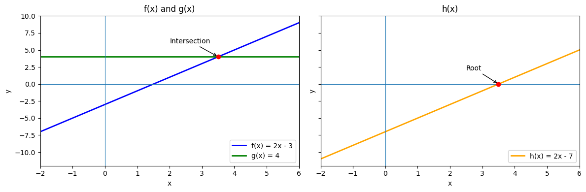
Consider the functions:

$f (x) = 2 x - 3 and g (x) = 4$

Here, $f (x)$ is linear and $g (x)$ is a constant function.

Finding the intersection of the graphs means determining $x$ such that:

$f (x) = g (x) \Leftrightarrow 2 x - 3 = 4$

We can convert this into a root-finding problem by moving all terms to one side, expressing the equation in the standard form $h (x) = 0$ :

$\Leftrightarrow \Leftrightarrow f (x) - g (x) 2 x - 3 - 4 2 x - 7 = 0 = 0 = 0$

Here, the left-hand side can be regarded as a new function $h (x) = 2 x - 7$ . Finding its root is equivalent to solving the original equation:

$\Leftrightarrow \Leftrightarrow \Leftrightarrow \Leftrightarrow \Leftrightarrow h (x) 2 x - 7 2 x \frac{2 x}{2} x x = 0 = 0 = 7 = \frac{7}{2} = \frac{7}{2} = 3.5$

The solution $x = 3.5$ represents the point where the graphs of $f (x)$ and $g (x)$ intersect. In terms of the root-finding approach, this is the zero of $h (x)$ , i.e., the value of $x$ for which $h (x)$ crosses the $x$ -axis.

Solving Quadratic Equations

In this section, we illustrate the equation-solving process for the case where the resulting difference $h (x) = f (x) - g (x)$ is quadratic. In such cases, solving $f (x) = g (x)$ is equivalent to finding the root of the quadratic function $h (x)$ .

Example: Roots of a Quadratic Function

*Left: Graphs of the given functions $f$ and $g$ . Right: Solving $f (x) = g (x)$ as a root-finding problem for the resulting quadratic function $h (x) = f (x) - g (x)$ .*

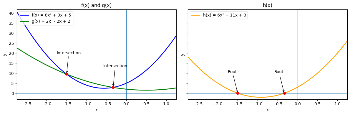
Consider the functions:

$f (x) = 8 x^{2} + 9 x + 5 and g (x) = 2 x^{2} - 2 x + 2$

Here, $f (x)$ and $g (x)$ are both quadratic.

Finding the intersection of the graphs means determining $x$ such that:

$f (x) = g (x) \Leftrightarrow 8 x^{2} + 9 x + 5 = 2 x^{2} - 2 x + 2$

We convert this to a root-finding problem by moving everything to one side:

$\Leftrightarrow \Leftrightarrow \Leftrightarrow f (x) - g (x) (8 x^{2} + 9 x + 5) - (2 x^{2} - 2 x + 2) 8 x^{2} + 9 x + 5 - 2 x^{2} + 2 x - 2 6 x^{2} + 11 x + 3 = 0 = 0 = 0 = 0$

At this stage, we have reduced the problem to solving a quadratic equation:

$h (x) = 6 x^{2} + 11 x + 3 = 0$

There are two standard ways to find its roots:

By factoring the quadratic expression into a product of two linear factors.
By applying the quadratic formula, which works even when factoring is not straightforward.

In the examples that follows, we will illustrate both approaches, using the same function $h (x)$ .

Solving Via Factorization

Factoring a quadratic expression means expressing it as a product of two linear factors. If this is possible, the zero product property can be applied:

$a \cdot b = 0 \Rightarrow a = 0 or b = 0$

This allows us to solve a quadratic equation by setting each factor equal to zero.

Example: Solving by Factorization

We are given the quadratic polynomial

$h (x) = 6 x^{2} + 11 + 3$

and want to factorize it using the grouping method, which we learned about in the previous Chapter 4.

The expression contains three terms, but the grouping method requires four. Thus, the first step is to rewrite the trinomial as a four-term polynomial. We can do this using Algorithm 1 from Chapter 4.

Step 1:: Identify coefficients:

$a = 6$ is the coefficient of the higest-order term $x^{2}$
$b = 11$ is the coefficient of the second-highest-order term $x$
$c = 3$ is the constant term

Step 2: Find two integers $m$ , $n$ such that

$m \cdot n = a \cdot c = 6 \cdot 3 = 18$
$m + n = b = 11$

Choosing $m = 9$ and $n = 2$ satisfies these conditions since $m \cdot n = 18$ and $m + n = 11$ .

Step 3: Rewrite the middle term using $m$ and $n$ : $6 x^{2} + 11 x + 3 = 6 x^{2} + m x 9 x + n x 2 x + 3$

Now we can apply the grouping method as described in Algorithm 2.

Step 1: Group the terms into pairs:

$(6 x^{2} + 9 x) + (2 x + 3)$

Step 2: Factor out the greatest common factor (GCF) from each group:

$3 x (2 x + 3) + 1 (2 x + 3)$

Step 3: A Common binomial factor appears:

$(2 x + 3) (3 x + 1) = 0.$

Finally, we can now apply the zero product property to solve for $x$ :

$2 x + 3 = 0 \Rightarrow x = - \frac{3}{2} and 3 x + 1 = 0 \Rightarrow x = - \frac{1}{3}$

Solving Via The Quadratic Formula

Another way to find the roots of $h (x)$ is to apply the quadratic formula.

Definition: The Quadratic Formula

Consider the quadratic equation:

$a x^{2} + b x + c = 0$

where $a \neq = 0$ . The solutions of this equation is given by the quadratic formula:

$x = \frac{- b \pm b ^{2} - 4 a c}{2 a}$

The discriminant $Δ = b^{2} - 4 a c$ determines the number of real solutions:

If $Δ > 0$ : two distinct real solutions.
If $Δ = 0$ : one real (repeated) solution.
If $Δ < 0$ : no real solutions.

Note: the $\pm$ symbol in the formula above means that we consider the expression both when the square root positive and negative.

Example: The Quadratic Formula

To solve the quardratic equation

$h (x) = 0 \Leftrightarrow 6 x^{2} + 11 + 3 = 0$

we set $a = 6$ , $b = 11$ , and $c = 3$ in the formula:

$x = \frac{- b \pm b ^{2} - 4 a c}{2 a} = \frac{- 11 \pm 1 1 ^{2} - 4 \cdot 6 \cdot 3}{2 \cdot 6} = \frac{- 11 \pm 121 - 72}{12} = \frac{- 11 \pm 49}{12}$

Hence, we get:

$x = \frac{- 11 + 7}{12} = - \frac{4}{12} = - \frac{1}{3} or x = \frac{- 11 - 7}{12} = - \frac{18}{12} = - \frac{3}{2}$

These match the solutions obtained by factoring.

Factorized Form and Roots of a Polynomial

Just as quadratic equations can be expressed in factorized form as

$f (x) = a (x - r_{1}) (x - r_{2})$

higher-order polynomials can likewise be written as a product of linear factors. This leads us to the following definition.

Definition: Factorized Form of a Polynomial

A polynomial function $f (x)$ of degree $n$ can be expressed as

$f (x) = a (x - r_{1}) (x - r_{2}) \dots (x - r_{n}),$

where $a$ is the leading coefficient and each $r_{i}$ is a root (or zero) satisfying $f (r_{i}) = 0$ .

This form reveals several geometric features of the polynomial:

The number of factors equals the degree of the polynomial
Each root $r_{i}$ corresponds to an $x$ -intercept of the graph
The coefficient $a$ determines the vertical stretch and orientation of the curve. For example, changing its sign reflects the graph across the $x$ -axis.

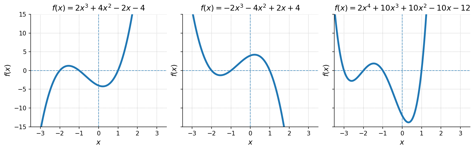
The following examples illustrate how these properties appear graphically.

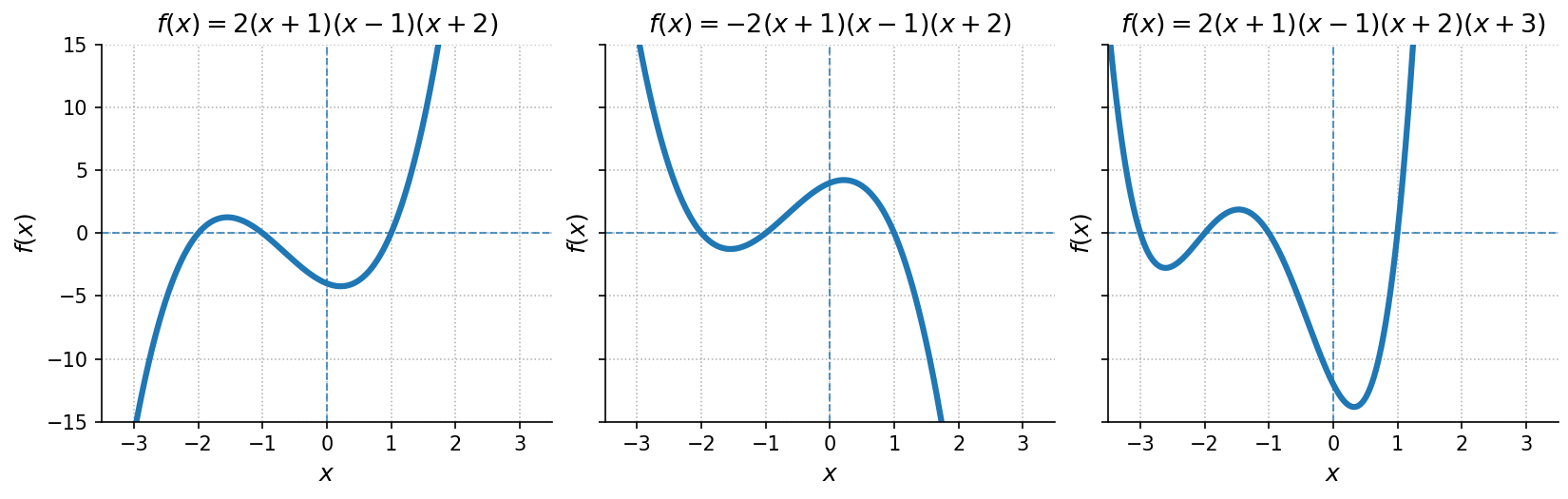
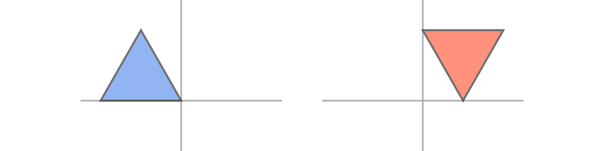
Examples: Factorized Form of a Polynomial

*Polynomials in factorized form. Each root $(x = r_{i})$ corresponds to an $x$ -intercept where $f (x) = 0$ .*

Consider the first polynomial in the plot:

$f (x) = 2 (x + 1) (x - 1) (x + 2)$

This function has three linear factors, so the polynomial is of degree three. The zeros, listed in the order they appear in the algebraic expression, are $x = - 1$ , $x = 1$ , and $x = - 2$ . At each of these points, one factor becomes zero, defining an $x$ -intercept where the graph meets the $x$ -axis.

Now look at the second polynomial in the plot:

$f (x) = - 2 (x + 1) (x - 1) (x + 2)$

The only difference is the sign of the leading coefficient. Changing it from $2$ to $- 2$ reflects the entire graph across the $x$ -axis, while the zeros remain in the same order and at the same positions.

Finally, consider the third polynomial in the plot:

$f (x) = 2 (x + 1) (x - 1) (x + 2) (x + 3)$

Here we have four linear factors, so the polynomial is of degree four. The zeros, again listed in the order of the factors, are $x = - 1$ , $x = 1$ , $x = - 2$ , and $x = - 3$ . As before, each root defines an $x$ -intercept where the graph meets the $x$ -axis.

The Sign and Behavior of a Function Around Its Roots

Finding the roots of a function does more than just tell us where it intercepts the $x$ -axis: It also reveals where the function takes on positive or negative values.

By analyzing the sign of $f (x)$ between its roots, we can determine on which intervals the function lies above or below the $x$ -axis, and thus describe its overall behavior.

The concepts of a function being Increasing on an Interval and Decreasing on an Interval further describe how the function behaves within those intervals, i.e., whether it rises or falls as $x$ changes.

These ideas are closely related: once the roots are known and the sign of $f (x)$ is determined, examining whether the function is increasing or decreasing helps us describe its overall shape and how it varies. Together, they provide a more complete picture of a function’s behavior, even without graphing it.

Definition: Positive and Negative Intervals

Let $f (x)$ be a real-valued function. We say that:

$f (x)$ is positive on an interval if $f (x) > 0$ for all $x$ in that interval.
$f (x)$ is negative on an interval if $f (x) < 0$ for all $x$ in that interval.

Graphically, this corresponds to whether the graph of the function lies above (positive) or below (negative) the $x$ -axis.

Because the sign of a function can only change at its roots, we can use the roots to divide the real line into intervals and then determine the sign of $f (x)$ within each one.

Example: Determining the Function Sign

For our quadratic function $h (x) = 6 x^{2} + 11 x + 3$ , we found earlier, that the roots are:

$x = - \frac{3}{2} and x = - \frac{1}{3} .$

These roots divide the real line into three intervals:

$(- \infty, - \frac{3}{2}), (- \frac{3}{2}, - \frac{1}{3}), (- \frac{1}{3}, \infty) .$

By testing a single point in each interval (for instance, $x = - 2, - 1, 0$ ), we find:

Interval	Test Value	Sign of $h (x)$	Behavior
$(- \infty, - \frac{3}{2})$	$x = - 2$	$h (- 2) = - 5 > 0$	$h (x)$ is positive
$(- \frac{3}{2}, - \frac{1}{3})$	$x = - 1$	$h (- 1) = - 2 < 0$	$h (x)$ is negative
$(- \frac{1}{3}, \infty)$	$x = 0$	$h (- 0) = - 3 > 0$	$h (x)$ is positive

Inverse Functions

When solving an equation of the form:

$f (x) = k$

we often want a general way to determine the input $x$ for any output value $k$ (in $f$ 's codomain). For some functions, it is possible to find another function that "reverses" the mapping performed by $f$ . This reversing function is called the inverse function.

Definition: Inverse of a Function

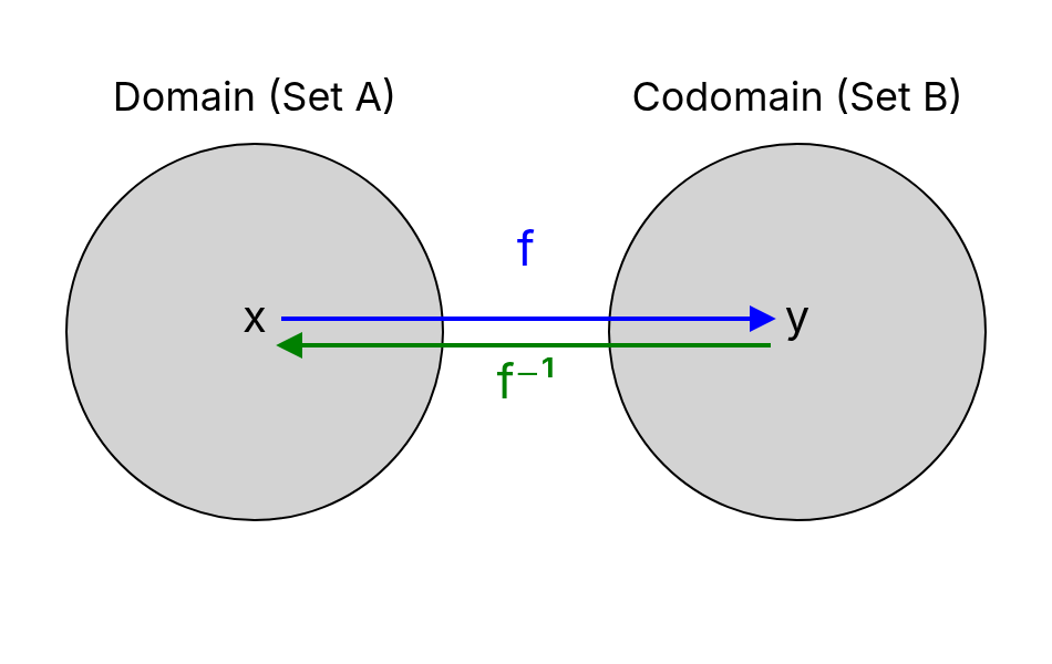
Let $f : A \to B$ be a function. An inverse function $f^{- 1} : B \to A$ satisfies:

$f^{- 1} (f (x)) = x and f (f^{- 1} (y)) = y$

for all $x \in A$ and $y \in B$ . This means that applying $f$ followed by $f^{- 1}$ (or vice versa) brings us back to the original value.

The inverse function essentially allows us to solve equations by applying $f^{- 1}$ to both sides:

$f (x) = y \Rightarrow \Leftrightarrow f^{- 1} (f (x)) x = f^{- 1} (y) = f^{- 1} (y)$

However, not every function has an inverse. Understanding when an inverse exists is thus essential.

Warning: Existence Conditions and Common Mistakes

A function $f$ has an inverse only if it is bijective, that is:
- Injective (one-to-one): no two inputs give the same output.
- Surjective (onto): every element of the codomain is produced by some input.
Otherwise, the mapping cannot be uniquely reversed.
The notation $f^{- 1}$ represents the inverse function, not the reciprocal: $f^{- 1} (x) \neq = \frac{1}{f ( x )} .$ The superscript $- 1$ indicates reversal of the mapping, not exponentiation.

Definition: Identity Property of Inverses

The composition of a function and its inverse returns the identity function on the respective domains:

$f \circ f^{- 1} = id_{B}, f^{- 1} \circ f = id_{A} .$

That is, the inverse of a function $f$ reverses the domain and codomain of $f$ . Graphically, the inverse corresponds to reflecting the graph of $f$ across the line $y = x$ .

Example: Finding an Inverse Function

Suppose $f : A \to B$ is defined by

$f (x) = 3 x + 5$

To find $f^{- 1}$ , solve for $x$ in terms of $y$ :

$y = 3 x + 5 \Leftrightarrow \Leftrightarrow y - 5 \frac{y - 5}{3} = 3 x = x$

This expression tells us how to recover $x$ from a given output $y$ , so:

$f^{- 1} (y) = \frac{y - 5}{3}$

Now, suppose we want to solve the equation:

$f (x) = 14$

To determine for which value of $x$ the function $f (x)$ is euqal to $14$ , we need to isolate $x$ on one side of the equality sign. Since we have already found the inverse of the function we can achieve this by applying $f^{- 1}$ to both sides:

$f^{- 1} (f (x)) = f^{- 1} (14)$

Since $f^{- 1}$ reverses the action of $f$ , the left-hand side simplifies to $x$ :

$x = \frac{14 - 5}{3} = 3$

In general, this is the reason for applying $f^{- 1}$ to both sides: it "undoes" $f$ on the side of the equality containing $x$ , essentially leaving $x$ alone.

Example: Verifying an Inverse Function

Consider the function in the earlier example, along with its inverse:

$f (x) = 3 x + 5 and f^{- 1} (y) = \frac{y - 5}{3}$

We can always check our work, by verifying the inverse properties, that is:

$f^{- 1} (f (x)) = x and f (f^{- 1} (y)) = y .$

Doing so, we indeed see that:

$f^{- 1} (f (x)) = f^{- 1} (3 x + 5) = \frac{( 3 x + 5 ) - 5}{3} = x$

Moreover, we see that:

$f (f^{- 1} (y)) = 3 (\frac{y - 5}{3}) + 5 = y$

Thus, $f (x) = 3 x + 5$ and $f^{- 1} (y) = \frac{y - 5}{3}$ are true inverses: each "undoes" the other's operation. In particular, $f$ multiplies by $3$ and adds $5$ , while $f^{- 1}$ subtracts $5$ and divides by $3$ , reversing the steps in the opposite order.

Common Inverses

Each of the examples given below show frequently used function-inverse pairs with their domains and ranges.

Example: Linear Shift

Example: Linear Scaling

Example: Power and Root Functions

Logarithm Rules

Since logarithms are inverse functions of exponentials, each rule in the table above can be derived directly from the exponent rules defined in Chapter 5.

Example: ...

Function $f (x)$	Inverse $f^{- 1} (x)$	Domain of $f$	Range of $f$
$f (x) = x + a$	$f^{- 1} (x) = x - a$	$R$	$R$
$f (x) = x - a$	$f^{- 1} (x) = x + a$	$R$	$R$
$f (x) = k x$ , $k \neq = 0$	$f^{- 1} (x) = \frac{x}{k}$	$R$	$R$
$f (x) = \frac{x}{k}$ , $k \neq = 0$	$f^{- 1} (x) = k x$	$R$	$R$
$f (x) = x^{n}$ , $n$ odd	$f^{- 1} (x) = n x$	$R$	$R$
$f (x) = x^{n}$ , $n$ even	$f^{- 1} (x) = n x$ (principal root)	$[0, \infty)$	$[0, \infty)$
$f (x) = e^{x}$	$f^{- 1} (x) = ln (x)$	$R$	$(0, \infty)$
$f (x) = a^{x}$ , $a > 0, a \neq = 1$	$f^{- 1} (x) = lo g_{a} (x)$	$R$	$(0, \infty)$
$f (x) = ln (x)$	$f^{- 1} (x) = e^{x}$	$(0, \infty)$	$R$
$f (x) = lo g_{a} (x)$ , $a > 0, a \neq = 1$	$f^{- 1} (x) = a^{x}$	$(0, \infty)$	$R$

Logarithm Rules

For $a > 0$ , $b > 0$ , $n \in R$ , and $a, b \neq = 1$ , the most important rules are given in the following table.

Rule	Formula	Description
Product Rule	$lo g_{b} (x \cdot y) = lo g_{b} (x) + lo g_{b} (y)$	The logarithm of a product equals the sum of the logarithms.
Quotient Rule	$lo g_{b} (\frac{x}{y}) = lo g_{b} (x) - lo g_{b} (y)$	The logarithm of a quotient equals the difference of the logarithms.
Power Rule	$lo g_{b} (x^{n}) = n \cdot lo g_{b} (x)$	A power in the argument becomes a multiplier in front of the logarithm.
Logarithm of 1	$lo g_{b} (1) = 0$	Any base raised to the power 0 equals 1.
Logarithm of the Base	$lo g_{b} (b) = 1$	Any base raised to the power 1 equals itself.
Inverse Property	$b^{l o g_{b} (x)} = x$	Exponential and logarithmic functions cancel each other.
Natural Log of $e$	$ln (e) = 1$	Since $ln (x)$ means $lo g_{e} (x)$ .
Change of Base	$lo g_{b} (x) = \frac{l o g _{k} ( x )}{l o g _{k} ( b )}$	Converts a logarithm from one base to another.

Note: The natural logarithm $ln (x)$ is simply $lo g_{e} (x)$ , where $e \approx 2.71828$ is Euler's number. All these rules work the same way for $ln$ as for $lo g_{b}$ for any base $b > 0$ , $b \neq = 1$ .

Since logarithms are inverse functions of exponentials, each rule in the table above can be derived directly from the exponent rules defined in Chapter 5.

Solving Non-Linear Equations

Many equations in mathematics involve non-linear functions such as exponentials and logarithms. The solving principles remain the same: we transform the equation into an equivalent one where the variable of interest is isolated, checking that the solution satisfies any domain restrictions.

A common strategy for solving these equations is to undo an operation using its inverse. In this context, we can make direct use of the inverse function pairs introduced earlier. In particular, when the variable appears in an exponent, we apply a logarithm to both sides, and when it appears inside a logarithm, we apply an exponential.

Example: Solving an Exponential Equation

Let us solve the equation $e^{2 x + 1} = w$ , $w > 0$ for $x$ .

$\Leftrightarrow \Leftrightarrow \Leftrightarrow e^{2 x + 1} ln (e^{2 x + 1}) 2 x + 1 x = w = ln (w) = ln (w) = \frac{1}{2} (ln (w) - 1)$

Example: Solving a Logarithmic Equation

Solve the equation $ln (x^{2} - 10) = 6$ for $x$ . Assume that $x^{2} > 10$ , as the logarithm otherwise is not defined. We obtain:

$\Leftrightarrow \Leftrightarrow \Leftrightarrow \Leftrightarrow ln (x^{2} - 10) e^{l n (x^{2} - 10)} x^{2} - 10 x^{2} x = 6 = e^{6} = e^{6} = e^{6} + 10 = \pm e^{6} + 10$

Determining Whether a Relation is a Function

Graphically

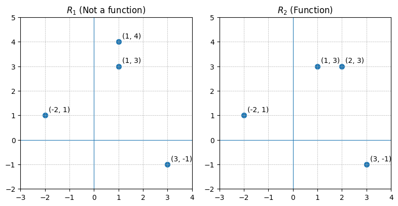
A relation in which each $x$ -coordinate is matched with exactly one $y$ -coordinate is said to describe $y$ as a function of $x$ . This also means that, if the same $x$ -coordinate is associated with two different $y$ -coordinates, then the relation is not a function.

Example: Checking Functional Relations

Which of the following relations descbribe $y$ as a function of $x$ ?

$R_{1} = {(- 2, 1), (1, 3), (1, 4), (3, - 1)}$
$R_{2} = {(- 2, 1), (1, 3), (2, 3), (3, - 1)}$

Inspecting the points of $R_{1}$ reveals that the $x$ -coordinate $1$ is matched with two different $y$ -coordinates: Namely $y = 3$ and $y = 4$ . Hence in $R_{1}$ , y is not a function of $x$ . On the other hand, every $x$ -coordinate in $R_{2}$ occurs only once which means each $x$ -coordinate has only one corresponding $y$ -coordinate. So, $R_{2}$ does represent $y$ as a function of $x$ . We can verify this graphically as well:

$R_{1} $ fails (same $x$ with different $y$ ); $R_{2}$ passes (each $x$ has one $y$ )

The Vertical Line Test

More generally, this also leads to the vertical line test, which is a quick graphical method to decide whether a relation is a function.

Definition: Vertical Line Test

Polynomial (function) passes the test; circle (not a function) fails. Intersection points are marked.

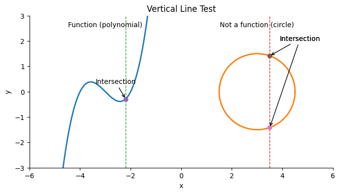
A relation is a function if and only if every vertical line intersects its graph at most once.

If a vertical line intersects more than once, the relation assigns more than one output to the same input thus violating the definition of a function.

It is important to note that equations can describe valid relationships—like the shape of a circle—but do not define a function. Recognizing this helps us understand both the limits of function notation and the situations where we need use other representations (such as parametric or implicit forms).

Algebraically

We can also check whether an equation defines a function by solving for one variable in terms of the other. If solving produces more than one output value for the same input, then the relation is not a function.

Example: Equation That Is Not a Function

Does the equation $x^{2} + y^{2} = 1$ represent a function with $x$ as input and $y$ as output? If so, express the relationship as a function $y = f (x)$ .

Solution:

First we subtract $x^{2}$ from both sides:

$y^{2} = 1 - x^{2}$

We now try to solve for $y$ in this equation:

$y = \pm 1 - x^{2}$

so, $y = 1 - x^{2}$ and $y = - 1 - x^{2}$ . We get two outputs corresponding to the same input, so this relationship cannot be represented as a single function $y = f (x)$ .

Chapter 5: Multivariable Functions

So far, we have focused on functions of a single variable, where each input is a single number $x$ and each output is a single number $y = f (x)$ . Many situations, however, involve relationships between more than one independent variable.

Examples: Multivariable Functions

For example:

The temperature at a given location may depend on both the latitude and the longitude
The profit of a company may depend on both the number of units sold and the unit price

When working with two independent variables, say $x$ and $y$ , it is natural to consider ordered pairs $(x, y)$ , where each coordinate is a real number. The set of all such pairs is denoted by $R^{2}$ and is often thought of as the Cartesian plane. Similarly, ordered triples $(x, y, z)$ form $R^{3}$ , which we interpret as three-dimensional space. More generally, $R^{n}$ denotes the set of all ordered $n$ -tuples $(x_{1}, x_{2}, \dots, x_{n})$ , where each coordinate is a real number.

Definition: Function of Several Variables

A real-valued function of $n$ variables is a rule that assigns to each input

$(x_{1}, x_{2}, \dots, x_{n}) \in A \subseteq R^{n}$

exactly one real number $f (x_{1}, x_{2}, \dots, x_{n}) \in R$ .

This is written as:

$f : A \to R$

The set $A$ is called the domain of $f$ and contains all valid inputs (points in $R^{n}$ ) for which $f$ is defined.
The range (or image) of $f$ is the set of all actual outputs: $Range (f) = {f (x_{1}, x_{2}, \dots, x_{n}) ∣ (x_{1}, x_{2}, \dots, x_{n}) \in A} .$

Visualizing Functions of Multiple Variables

When $n = 1$ , the graph of a function $f (x)$ can be drawn in a two-dimensional coordinate system. When $n = 2$ , we can represent the graph in three dimensions, with the third axis showing the value of $f (x, y)$ . For $n \geq 3$ , it is no longer possible to directly visualize the graph in physical space, but other techniques, such as level curves and function traces, can be used to represent the function’s behavior.

To illustrate these ideas, we extend the crop yield model we studied earlier, in Chapter 3, to include additional factors.

Example: Extended Crop Yield Model

In reality, crop yield depends on more than just fertilizer amount. Another important factor is rainfall, denoted by $y$ (in millimeters over a growing season of about $120$ days, i.e., $\approx 4$ months). We now model crop yield as a function of two variables:

$f (x, y) = crop yield for fertilizer x and rainfall y$

Here, $f : R^{2} \to R$ assigns a real-valued yield to each ordered pair $(x, y)$ within a suitable domain (e.g., $x > 0$ kg/ha of fertilizer and $y > 0$ mm of rainfall).

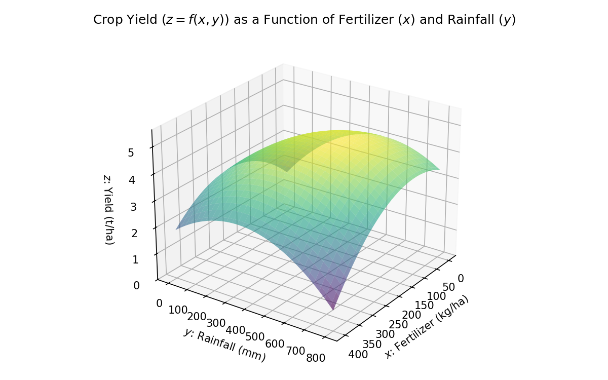
Graph of the crop yield $z = f (x, y)$ as a function of fertilizer $x$ and rainfall $y$ .

Because $f$ depends on two variables, its graph lives in three dimensions: the horizontal plane represents $x$ (fertilizer) and $y$ (rainfall), while the vertical axis represents $f (x, y)$ (yield). Although 3D graphs are possible, they can be difficult to interpret—especially for decision-making—so we often use level curves and function traces instead.

Level Curves or Contours

Level curves show where the function has the same value, making it easier to identify trade-offs and regions of interest.

Definition: Level Curve of a Function

For a function of two variables $f (x, y)$ , a level curve (or contour) is the set of all points $(x, y)$ in the domain where the function takes a fixed constant value $k$ :

$f (x, y) = k$

In the $x y$ -plane, a level curve connects all points where $f$ produces the same output.

In the crop yield model, a level curve for $f$ represents all combinations of fertilizer and rainfall that yield the same harvest.

For a fixed yield $z_{0}$ , the level curve is:

${(x, y) ∣ f (x, y) = z_{0}}$

For example, the level curve for $f (x, y) = 4.4 t/ha$ shows all fertilizer-rainfall combinations producing a yield of $4.4$ tonnes per hectare.

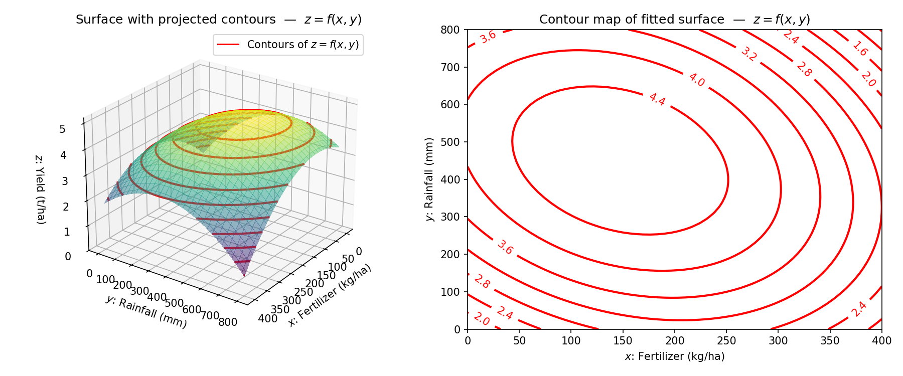
From a contour plot, we can answer questions such as:

"If I want $4.4$ t/ha, how can I trade fertilizer for rainfall?"
"Where is the optimal combination of fertilizer and rainfall for maximum yield?"

Level curves are especially useful for visualizing decision boundaries and trade-offs when multiple factors influence an outcome.

Function Traces

Function traces help us examine cross-sections of the surface by fixing one variable and varying the other.

Definition: Trace of a Function

For $f (x, y)$ , a trace is obtained by fixing one variable and letting the other vary:

Trace in the $x$ -direction: Fix $y = c$ and consider $z = f (x, c)$

This curve lies in the vertical plane parallel to the $x z$ -plane.

Trace in the $y$ -direction: Fix $x = c$ and consider $z = f (c, y)$

This curve lies in the vertical plane parallel to the $yz$ -plane.

For example:

Fix fertilizer at $150$ kg/ha and vary rainfall: The trace shows how yield changes with rainfall for that fertilizer level.

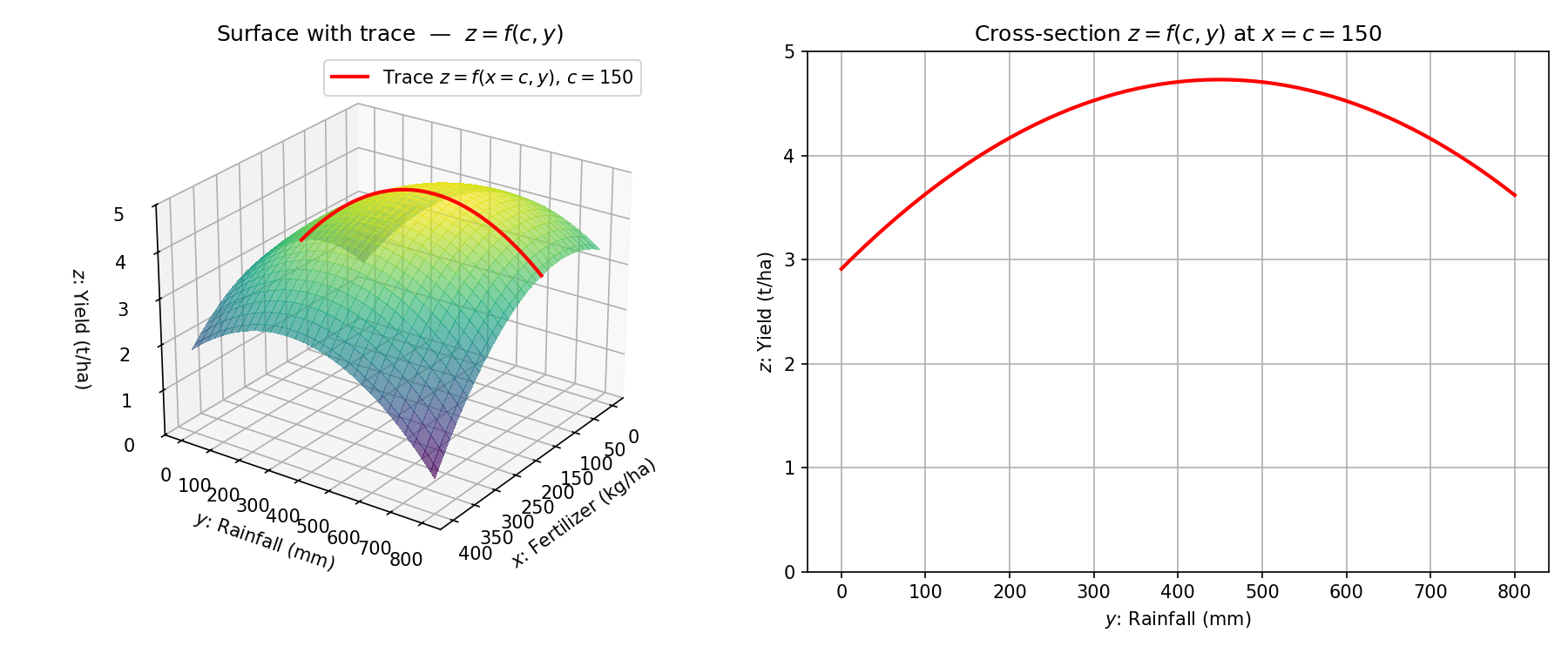
Trace: Yield vs Rainfall with Fertilizer fixed at $150$ kg/ha.
Fix rainfall at $450$ mm and vary fertilizer: The trace shows how yield changes with fertilizer for that rainfall level.

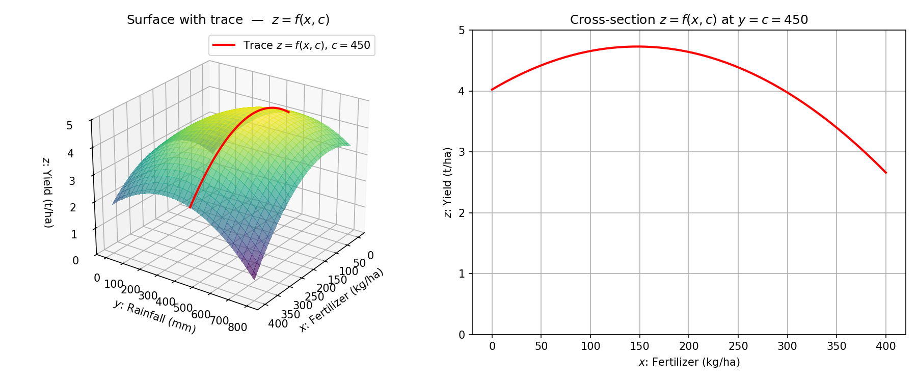
Trace: Yield vs Fertilizer with Rainfall fixed at $450$ mm.

From these traces, we can identify tipping points, such as the fertilizer amount beyond which adding more no longer increases yield.

Computing Level Curves and Traces

The task of finding level curves and traces reduces to solving equations. The algebraic and graphical techniques are the same as those used for curves in two dimensions, but here they are applied to cross-sections and slices of surfaces.

Examples: ???

Find the domain and range of each of the following functions:

$f (x, y) = 3 x + 5 y + 2$
$g (x, y) = 9 - x^{2} - y^{2}$

Chapter 6: Limits

Limits & Continuity

The concept of a limit concerns the value that a function approaches as its input gets closer to a particular point. Importantly, what happens exactly at that point is not what matters, instead, we focus on what happens around the point.

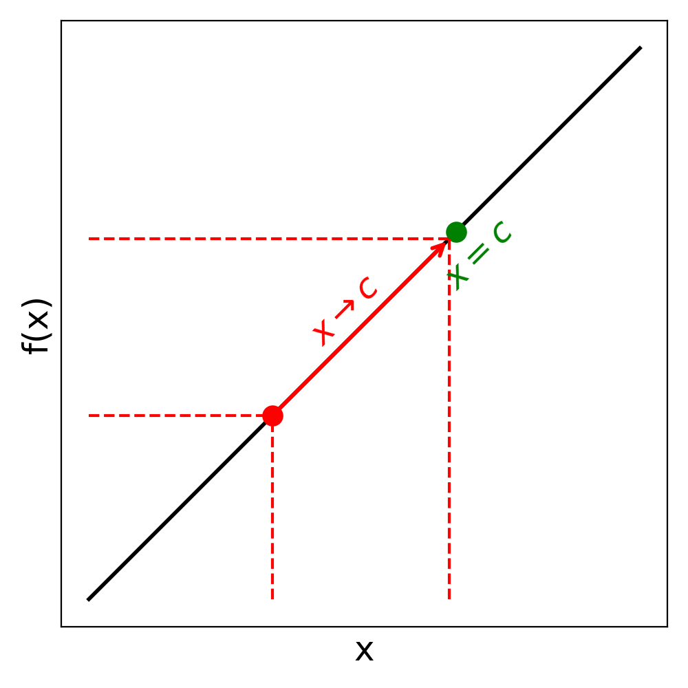
Understanding the concept of a limit is fundamental as it allows us to study the continuity of functions, a property describing whether a function behaves smoothly without abrupt jumps or breaks. Furthermore, limits are the foundation for defining derivatives, which describe rates of change.

Example 1: Limits

To illustrate this and build an intuitive understanding of the concept of limit, consider the function and its corresponding graph:

$f (x) = ⎩ ⎨ ⎧ x^{2}, 2, sin (x), x \in [0, 1) x \in [1, π) x \in [π, 2 π]$

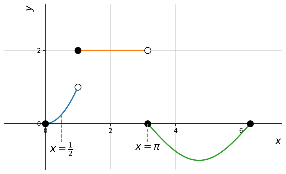
Let us consider the limit of $f (x)$ as $x \to \frac{1}{2}$ . This means that we look at values of $f (x)$ for $x$ in some small interval around $\frac{1}{2}$ . In this case, this corresponds to examining the function $x^{2}$ on the interval $[0, 1)$ . If we look the graph of this function, we can see that as $x$ approaches $\frac{1}{2}$ from either the left or the right, the value of $f (x)$ approaches $\frac{1}{4}$ .

Therefore, the limit of $f (x)$ as $x \to \frac{1}{2}$ can be expressed symbolically as:

$x \to \frac{1}{2} lim f (x) = \frac{1}{4}$

This example illustrates the basic idea behind limits. We now state this idea in more general terms.

Definition: Limit

Let $f (x)$ be a function defined on an open interval containing $a$ (with the possible exception of $a$ itself). Let $L$ be a real number. If all values of the function $f (x)$ approach the real number $L$ as the values of $x \neq = a$ approach the number $a$ , then we say that the limit of $f (x)$ as $x$ approaches $a$ is $L$ .

In words, as $x$ gets closer to $a$ , $f (x)$ gets closer and stays close to $L$ . Symbolically, we express this idea as

$x \to a lim f (x) = L$

if and only if

$x \to a^{+} lim f (x) = L and x \to a^{-} lim f (x) = L .$

Here $x \to a^{+}$ means approaching $a$ from the right (positive direction) and $x \to a^{-}$ means approaching from the left (negative direction).

Example 2: Limits

Not every function has a limit at every point. A limit may fail to exist for several reasons. To illustrate this, we return to our earlier example and now consider $x = 1$ and $x = π$ . At each of these points, the left-hand and right-hand limits differ:

$L^{-} = x \to π^{+} lim f (x) = 2 and L^{+} = x \to π^{-} lim f (x) = 0$

Since these one-sided limits are not equal, $x \to π lim f (x)$ does not exist. The same reasoning applies at $x = 1$ .

Another way a limit can fail to exist is if the function grows without bound, for example:

$x \to \infty lim x^{2}$

As $x$ increases, $x^{2}$ grows without limit, so it does not approach a finite value. We may write $x^{2} \to \infty$ as $x \to \infty$ , but the limit does not exist in the finite sense.

Discontinuity

A discontinuity is a point where the function’s value changes abruptly. In our first example, $f$ has discontinuities at $x = 1$ and $x = π$ because the limits at these points do not exist.

Example: ...

Consider the function shown below, where $f$ has jumps at $x = 1$ and $x = π$ .

At $x = π$ , the one-sided limits are different:

$x \to π^{-} lim f (x) = 0 and x \to π^{+} lim f (x) = 2$

Because the left-hand and right-hand limits do not agree,
the two-sided limit $lim_{x \to π} f (x)$ does not exist.
Therefore, $f$ has a jump discontinuity at $x = π$ .

However, discontinuity does not always mean the limit fails to exist. For instance, consider the following example.

Example 3: Limits

$f (x) = {- x^{2} + 2, 1, x \in R ∖ {0} x = 0$

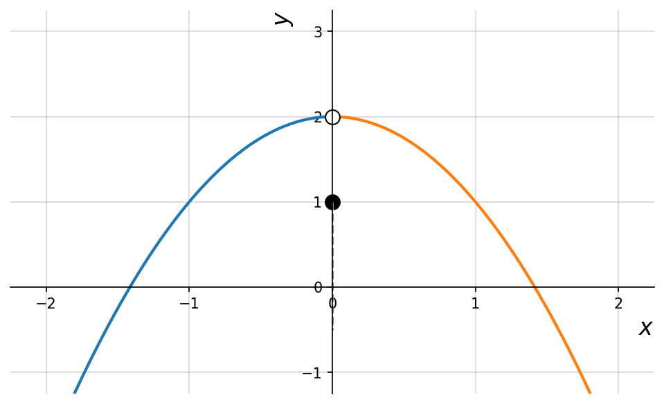
Looking at the graph, it is clear that despite $lim_{x \to 0} f (x) = 2$ , the actual function value is $f (0) = 1$ . In this case, we say that $f$ is discontinuous at $x = 0$ .

Continuity

The discussion about when limits exist and do not exist, leads us to the following definition.

Definition: Continuity

Let $f : D \to R$ be a function, where $D \subseteq R$ is the domain of $f$ .

The function $f$ is said to be continuous at a point $c \in D$ if

$x \to c lim f (x) = f (c)$

That is, as $x$ approaches $c$ , the value of $f (x)$ approaches the same number that $f$ actually takes at $c$ .

Breaking this definition into its essential parts:

The limit exists:
The left-hand and right-hand limits of $f (x)$ at $c$ are equal.
In symbols,

$x \to c^{-} lim f (x) = x \to c^{+} lim f (x) = L$

This ensures that $f (x)$ approaches a single, well-defined value near $c$ .
The function value is defined:
The point $f (c)$ exists, meaning that $c$ belongs to the domain $D$ .
Without a defined value at $c$ , the concept of continuity cannot apply.
The limit equals the function value:
The value that $f (x)$ approaches near $c$ is exactly the same as the value it takes at $c$ :

$L = f (c)$

This guarantees there is no jump or gap in the function’s behavior at that point.

If $f$ is continuous at every point $c \in D$ , then we say that $f$ is continuous on $D$ .

Continuity can therefore be viewed as a local property at each point, which extends to a global property when it holds throughout the entire domain.

In practice, most functions we encounter (such as polynomial, exponential, logarithmic, and trigonometric functions) are continuous on the domains we care about.

Example: ...

Consider the function

$f (x) = {- x^{2} + 2, 1, x \in R ∖ {0} x = 0$

We want to determine whether $f$ is continuous at $x = 0$ .

The limit exists:

$x \to 0^{+} lim f (x) = 2 and x \to 0^{-} lim f (x) = 2$

Since both one-sided limits are equal, the limit $lim_{x \to 0} f (x)$ exists and equals 2. The condition is satisfied.
The function value is defined:

$f (0) = 1$

The function has a defined value at $x = 0$ . The condition is satisfied.
The limit equals the function value:

$x \to 0 lim f (x) = 2 \neq = f (0) = 1$

The limit and the function value are not equal. The condition is not satisfied.

Since the third condition fails, $f$ is not continuous at $x = 0$ .

Limit Laws

In an earlier chapter, we saw how to combine two functions using arithmetic operations. The table below shows the corresponding rules for limits, assuming both $x \to a lim f (x)$ and $x \to a lim g (x)$ exist.

Table 1. ...

Operation	Limit Law
Constant Multiple	$x \to a lim [c \cdot f (x)] = c \cdot x \to a lim f (x)$
Sum/Difference	$x \to a lim [f (x) \pm g (x)] = x \to a lim f (x) \pm x \to a lim g (x)$
Product	$x \to a lim [f (x) \cdot g (x)] = x \to a lim f (x) \cdot x \to a lim g (x)$
Quotient	$x \to a lim \frac{f ( x )}{g ( x )} = \frac{lim _{x \to a} f ( x )}{lim _{x \to a} g ( x )}, x \to a lim g (x) \neq = 0$

Example 1: ...

Determine $lim_{x \to 1} (x + 3 - 4 - x)$

Split into two limits (use the difference law):

$x \to 1 lim x + 3 - x \to 1 lim 4 - x$

Evaluate each part directly (direct substitution):

$x \to 1 lim x + 3 - x \to 1 lim 4 - x = 1 + 3 - 4 - 1 = 4 - 3 = 2 - 3$

Example 2: ...

Determine $lim_{x \to 1} \frac{x ^{2} - 1}{x - 1}$

Check direct substitution (does not work!):

$\frac{1 ^{2} - 1}{1 - 1} = \frac{0}{0}$

Factor numerator and cancel the common factor:

$x \to 1 lim \frac{x ^{2} - 1}{x - 1} = x \to 1 lim \frac{( x - 1 ) ( x + 1 )}{x - 1} = x \to 1 lim x + 1$

Evaluate the expression (direct subsitution):

$x \to 1 lim x + 1 = 1 + 1 = 2$

Chapter Exercise

Chapter 7: Differentiation

Differentiation

Differentiation is the process of finding the derivative of a function, which tells us the slope of the function at a single point on its graph.

In an earlier chapter, we defined the slope in the context of a linear function. To extend this concept to more general functions, we first define secant lines (slopes over an interval) and then tangent lines (slopes at a single point). These ideas allow us to quantify how a function changes.

Secant & Tangent Lines

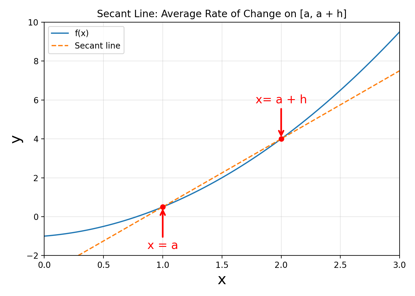
The slope of a secant line to a function at a point $(a, f (a))$ gives an average rate of change of a function between $x = a$ and a nearby point.

To compute it, we pick a value of $x$ close to $a$ , say $x = a + h$ (where $h \neq = 0$ ), and draw a line through the points $(a, f (a))$ , and $(a + h, f (a + h))$ . The slope of this line is:

$m_{sec} = \frac{f ( x ) - f ( a )}{x - a} = \frac{f ( a + h ) - f ( a )}{( a + h ) - a} = \frac{f ( a + h ) - f ( a )}{h}$

Definition: Slope of a Secant Line

Let $f$ be a function defined on an interval $I$ containing $a$ . If $h \neq = 0$ and $a + h \in I$ , the slope of the secant line is:

$m_{sec} = \frac{f ( a + h ) - f ( a )}{h} .$

This expression is also called the difference quotient.

Example: Slope of a Secant Line

Find the slope of the tangent line to the graph of $f (x) = x^{2}$ at $x = 3$ .

$m_{t an} = h \to 0 lim \frac{f ( 3 + h ) - f ( 3 )}{h} = h \to 0 lim \frac{( 3 + h ) ^{2} - 9}{h} = h \to 0 lim \frac{9 + 6 h + h ^{2} - 9}{h} = h \to 0 lim \frac{h ( 6 + h )}{h} = h \to 0 lim 6 + h = 6$

Definition: Tangent Line

Let $f (x)$ be a function defined in an open interval containing $a$ . The tangent line to $f$ at $x = a$ is the line passing through $(a, f (a))$ with slope:

$m_{tan} = h \to 0 lim \frac{f ( a + h ) - f ( a )}{h}$

provided this limit exists.

Example: Tangent Line

Find the slope of the tangent line to the graph of $f (x) = x$ at $x = 4$ .

$m_{tan} = h \to 0 lim \frac{f ( 4 + h ) - f ( 4 )}{h} = h \to 0 lim \frac{4 + h - 4}{h} = h \to 0 lim (\frac{4 + h + 2}{4 + h + 2}) \cdot \frac{4 + h - 2}{h} = h \to 0 lim \frac{( 4 + h + 2 ) \cdot ( 4 + h - 2 )}{( 4 + h + 2 ) \cdot h} = h \to 0 lim \frac{4 + h ^{2} - 2 ^{2}}{( 4 + h + 2 ) \cdot h} = h \to 0 lim \frac{4 + h - 4}{( 4 + h + 2 ) \cdot h} = h \to 0 lim \frac{h}{( 4 + h + 2 ) \cdot h} = h \to 0 lim \frac{1}{4 + h + 2} = \frac{1}{4 + 2} = \frac{1}{2 + 2} = \frac{1}{4}$

The Derivative of a Function

Definition: The Derivative of a Function

Let $f : (a, b) \to R$ be a function. The derivative of $f$ at $x$ is:

$f^{'} (x) = h \to 0 lim \frac{f ( x + h ) - f ( x )}{h}$

provided the limit exists. If the limit exists for all $x \in (a, b)$ , we say that $f$ is differentiable on $(a, b)$ .

Note that instead of writing $f^{'} (x)$ , we can also write $\frac{df}{d x}$ or $\frac{d}{d x} f (x)$ . All three expressions denote the derivative of $f$ with respect to $x$ .

The prime notation $f^{'} (x)$ is concise and often used in basic calculus or when the variable is clear from context.

The Leibniz notation $\frac{df}{d x}$ , on the other hand, emphasizes the operation of differentiation and explicitly indicates the variable, making it useful in contexts with, e.g., several variables or when applying rules like the chain rule.

Note that instead of writing $f^{'} (x)$ we sometimes write $\frac{df}{d x}$ or $\frac{d}{d x} f (x)$ , i.e., these expressions are equivalent, but ...

Example: The Derivative of a Linear Function

Consider the linear function $f (x) = a x + b, a \neq = 0, b \in R$ . For any $x \in R$ . We compute the derivative of the function, as follows:

$f^{'} (x) f^{'} (x) f^{'} (x) f^{'} (x) = h \to 0 lim \frac{( a ( x + h ) + b ) - ( a x + b )}{h} = h \to 0 lim \frac{( a x + ah + b ) - ( a x + b )}{h} = h \to 0 lim \frac{a x + ah + b - a x - b}{h} = h \to 0 lim \frac{ah}{h} = h \to 0 lim a = a$

This makes sense, as a linear function is a straight line with constant slope.

Example: The Derivative of a Quadratic Function

Consider the quadratic function $f (x) = a x^{2}$ , for any $x \in R$ . We compute the derivative of the function, using the limit laws, as follows:

$f^{'} (x) = h \to 0 lim \frac{a ( x + h ) ^{2} - a x ^{2}}{h} = a \cdot n \to \infty lim \frac{( x + h ) ^{2} - x ^{2}}{h} = a \cdot h \to 0 lim \frac{x ^{2} + h ^{2} + 2 h x - x ^{2}}{h} = a \cdot h \to 0 lim \frac{h ^{2} + 2 h x}{h} = a \cdot h \to 0 lim \frac{h ( h + 2 x )}{h} = a \cdot h \to 0 lim h + 2 x = 2 a x$

Common Derivatives

Below is a table of some of the most frequently used derivatives. Here $k, a \in R$ , $a > 0$ , and $n \neq = 0$ .

Function $f (x)$	Derivative $f^{'} (x)$	Notes
$k$	$0$	Constant rule
$x^{n}$	$n x^{n - 1}$	Power rule
$ln (x)$	$\frac{1}{x}$	$x > 0$
$e^{x}$	$e^{x}$	-
$a^{x}$	$ln (a) a^{x}$	$a > 0$
$sin (x)$	$cos (x)$	-
$cos (x)$	$- sin (x)$	-

Example: ...

Using the rules in the table, compute the derivative of the function $h (x) = e^{x} sin (x)$ .

Letting $f (x) = e^{x}$ and $g (x) = sin (x)$ , we get from the table of derivatives that $f^{'} (x) = e^{x}$ and $g^{'} (x) = cos (x)$ . The product rule then gives

$h^{'} (x) = \frac{d}{d x} (e^{x} sin (x)) = e^{x} sin (x) + e^{x} cos (x) = e^{x} (sin (x) + cos (x))$

Common Differentiation Rules

Just like for limits, there are certain rules that we can apply when differentiating functions. In this context, let $f$ and $g$ be differentiable functions on an interval, with $g (x) \neq = 0$ . The following rules then hold:

Rule	Formula	Name
Sum/Difference	$\frac{d}{d x} (f (x) \pm g (x)) = f^{'} (x) \pm g^{'} (x)$	Sum/Difference Rule
Product	$\frac{d}{d x} (f (x) g (x)) = f^{'} (x) g (x) + f (x) g^{'} (x)$	Product Rule
Quotient	$\frac{d}{d x} (\frac{f ( x )}{g ( x )}) = \frac{f ^{'} ( x ) g ( x ) - f ( x ) g ^{'} ( x )}{( g ( x ) ) ^{2}}$	Quotient Rule
Constant Multiple	$\frac{d}{d x} (k f (x)) = k f^{'} (x), k \in R$	Constant Multiple Rule

Example:

Differentiate the functions $f (x) = 2 x^{2}$ , $g (x) = x$ , and consider the derivative of the product $f (x) \cdot g (x)$ and the quotient $\frac{f ( x )}{g ( x )}$ , without performing algebraic manipulations until the very end.

We already know that

$f^{'} (x) = \frac{d}{d x} (2 x^{2}) = 2 \cdot 2 \cdot x = 4 x and g^{'} (x) = \frac{d}{d x} (x) = 1$

Now, computing the product, we get:

$(f (x) g (x))^{'} = \frac{d}{d x} (f (x) g (x)) = f^{'} (x) g (x) + f (x) g^{'} (x) = 4 x \cdot x + 2 x^{2} \cdot 1 = 6 x^{2}$

For the quotient, where we assume $x \neq = 0$ , as $g (x)$ otherwise would be zero, we get:

$(\frac{f ( x )}{g ( x )})^{'} = \frac{d}{d x} \frac{f ( x )}{g ( x )} = \frac{4 x \cdot x - 2 x ^{2} \cdot 1}{x ^{2}} = \frac{2 x ^{2}}{x ^{2}} = 2$

The Chain Rule

We have seen the techniques for differentiating basic functions as well as sums, differences, products, quotients, and constant multiples of these functions. However, these techniques do not allow us to differentiate compositions of functions. In this section, we study the rule for finding the derivative of the composition of two or more functions.

Definition: The Chain Rule

Let $f$ and $g$ be functions such that:

$g$ is differentiable at $x$
$f$ is differentiable at $g (x)$

For the composite function:

$h (x) = (f \circ g) (x) = f (g (x))$

the derivative is then defined as:

$\frac{d}{d x} (f \circ g) (x) = f^{'} (g (x)) \cdot g^{'} (x)$

Recipie: Applying the Chain Rule

To differentiate $h (x) = f (g (x))$ , follow the steps:

Identify the outer function $f (x)$ and the inner function $g (x)$
Differentiate $f$ with respect to its argument to get $f^{'} (x)$
Evaluate $f^{'} (g (x))$ by substituting $g (x)$ into $f^{'} (x)$
Differentiate $g$ with respect to its argument to get $g^{'} (x)$
Compute $h^{'} (x)$ as $f^{'} (g (x)) \cdot g^{'} (x)$

Definition:

Differentiate $h (x) = (sin (x))^{2}$ .

To do so, we let:

The outer function be $f (u) = u^{2}$ , so $f^{'} (u) = 2 u$
The inner function be $g (x) = sin (x)$ , so $g^{'} (x) = cos (x)$

Applying the Chain Rule, we then get:

$h^{'} (x) = f^{'} (g (x)) \cdot g^{'} (x) = 2 sin (x) \cdot cos (x)$

Example:

Differentiate $f (x) = e^{x^{3} + 1}$ .

To do so, we let:

The outer function be $f (u) = e^{u}$ , so $f^{'} (u) = e^{u}$ .
The inner function be $g (x) = x^{3} + 1$ , so $g^{'} (x) = 3 x^{2}$ .

Applying the Chain Rule, we then get:

$f^{'} (x) = e^{x^{3} + 1} \cdot 3 x^{2} = 3 x^{2} e^{x^{3} + 1} .$

Finding Extrema

In this section, we focus on an important application of derivatives: finding maxima and minima of functions.

Definition: Local Minima and Maxima

Let $f$ be defined on an interval $I$ containing $x$ , then:

$f (c)$ is the minimum of $f$ on $I$ if $f (c) \leq f (x)$ for all $x \in I$
$f (c)$ is the maximum of $f$ on $I$ if $f (c) \geq f (x)$ for all $x \in I$

The maximum and minimum values are the extreme values, or extrema, of $f$ on $I$ .

Definition: The Extreme Value Theorem

Let $f$ be a continuous function defined on a closed interval $I$ . Then $f$ has both a maximum and minimum value on $I$ .

The Turning Point of a Quadratic Function

Recall from earlier, a turning point (or tipping point) of a graph is a point at which the graph changes direction from increasing to decreasing or vice versa. For a quadratic formula, the formula for the turning point is:

$T = (- \frac{b}{2 a}, - \frac{Δ}{4 a}), with Δ = b^{2} - 4 a c$

We will later see how to find derive this point by setting the first derivative of the function to zero and solving for $x$ (i.e., $f^{'} (x) = 0$ ).

For $h (x) = 6 x^{2} + 11 x + 3$ , with discriminant $D = 49$ , the turning point is:

$x_{T} y_{T} = - \frac{b}{2 a} = - \frac{11}{2 \cdot 6} = - \frac{11}{12} \approx - 0.917 = - \frac{D}{4 a} = - \frac{49}{4 \cdot 6} = - \frac{49}{24} \approx - 2.042$

Since $a = 6 > 0$ , the parabola opens upwards, and the turning point is a minimum. This can also be confirmed by inspecting the graph.

Derivatives & Local Extrema

The derivative $f^{'} (x)$ measures the slope of the tangent line at $(x, f (x))$ . At a local maximum or minimum, the tangent line is horizontal, meaning:

$f^{'} (x_{0}) = 0 or f^{'} (x_{0}) is undefined$

Such points are also called critical points.

Definition: The Second Derivative Test

Let $f$ be a 2-times differentiable function and $x_{0}$ a point such that $f^{'} (x_{0}) = 0$ . Then

If $f^{''} (x_{0}) > 0$ we have a local minimum
If $f^{''} (x_{0}) < 0$ we have a local maximum
If $f^{''} (x_{0}) = 0$ or doesn't exist, the test gives no information

Example: Finding Local Maxima and Minima

Find the local maxima and minima of the function $f (x) = 2 x^{3} + \frac{3}{4} x^{2} - \frac{5}{2} x$ .

We differentiate $f$ and obtain

$f^{'} (x) = 6 x^{2} + 2 \cdot \frac{3}{4} x - \frac{5}{2} = 6 x^{2} + \frac{3}{2} x - \frac{5}{2}$

In order to find the points where $f^{'} (x) = 0$ we solve the quadratic equation $6 x^{2} + \frac{3}{2} x - \frac{5}{2} = 0$ . The discriminant is $D = (\frac{3}{2})^{2} - 4 \cdot 6 \cdot (- \frac{5}{2}) = \frac{249}{4}$ and the roots are thus

$x_{1} x_{2} = \frac{- \frac{3}{2} - \frac{249}{4}}{2 \cdot 6} \approx 0.53, = \frac{- \frac{3}{2} + \frac{249}{4}}{2 \cdot 6} \approx - 0.78$

Differentiating once again, we obtain

$f^{''} (x) = 12 x + \frac{3}{2}$

and by calculation, $f^{''} (x_{1}) > 0$ and $f^{''} (x_{2}) < 0$ . We can compute the coordinates $(x_{1}, f (x_{1})) = (0.53, - 0.81)$ , $(x_{2}, f (x_{2})) = (- 0.78, 1.45)$

Chapter Exercises

Chapter 9: Sequences, Sums & Products

This chapter introduces notation for working with ordered lists of numbers and with repeated addition or multiplication. These ideas appear throughout mathematics whenever we want to describe a pattern compactly instead of writing out every term.

Sequences

A sequence is an ordered list of numbers. For example, the numbers

$0, 1, 2, 3, 4, 5, \dots$

form a sequence. This is different from a set because, in a sequence, the order of the terms matters. For this reason, when we use variables to represent terms in a sequence, we attach an index to each term:

$a_{0}, a_{1}, a_{2}, a_{3}, \dots$

The numbers in the subscripts are called indices (the plural of index).

Definition: Sequence

A sequence is an ordered list of numbers. We often denote the entire sequence by

${a_{n}}_{n = 0}^{\infty},$

where $a_{n}$ is the term with index $n$ .

Summation Notation

Given a sequence ${a_{n}}_{n = k}^{\infty}$ and numbers $m$ and $p$ satisfying $k \leq m \leq p$ , the summation from $m$ to $p$ of the sequence ${a_{n}}$ is written

$n = m \sum p a_{n} = a_{m} + a_{m + 1} + \dots + a_{p} .$

The variable $n$ is called the index of summation. The number $m$ is called the lower limit of summation, while the number $p$ is called the upper limit of summation.

Example: Expanding a Sum

Suppose we have the sequence $a_{n} = 2 n - 1$ for $n \geq 1$ . We can write the sum

$a_{3} + a_{4} + a_{5} + a_{6}$

$n = 3 \sum 6 (2 n - 1) = = = (2 (3) - 1) + (2 (4) - 1) + (2 (5) - 1) + (2 (6) - 1) 5 + 7 + 9 + 11 32.$

The index variable is considered a "dummy variable" in the sense that it may be changed to any letter without affecting the value of the summation. For instance,

$n = 3 \sum 6 (2 n - 1) = k = 3 \sum 6 (2 k - 1) = j = 3 \sum 6 (2 j - 1) .$

One place you may encounter summation notation is in mathematical definitions. For example, summation notation allows us to define polynomials as functions of the form:

$f (x) = a_{n} x^{n} + a_{n - 1} x^{n - 1} + \dots + a_{1} x + a_{0} = k = 0 \sum n a_{k} x^{k} .$

Here:

$n$ is a non-negative integer (the degree of the polynomial).
$a_{n}, a_{n - 1}, \dots, a_{0}$ are real constants.
$a_{n} \neq = 0$ if $n > 0$ .

Example: Evaluating and Writing Sums

Find the following sum:

$k = 1 \sum 3 \frac{7}{1 0 ^{k}}$

Expanding the notation gives

$k = 1 \sum 3 \frac{7}{1 0 ^{k}} = = = \frac{7}{1 0 ^{1}} + \frac{7}{1 0 ^{2}} + \frac{7}{1 0 ^{3}} 0.7 + 0.07 + 0.007 0.777.$

The sum

$1 + 3 + 5 + \dots + 117$

can be written using summation notation as

$k = 1 \sum 59 (2 k - 1) .$

Example: More Summation Practice

Find the following sum:

$1 + 2 + 3 + 4 + 5 = 15.$

The sum

$2 + 4 + 6 + 8 + 10$

can be written as

$k = 1 \sum 5 2 k .$

Finally, evaluate the following sum:

$k = 1 \sum 4 (2 k + 1)$

Expanding the terms gives

$k = 1 \sum 4 (2 k + 1) = (2 (1) + 1) + (2 (2) + 1) + (2 (3) + 1) + (2 (4) + 1) = 3 + 5 + 7 + 9 = 24.$

Product Notation

If we want to multiply elements of a sequence instead of adding them, we use product notation.

Given a sequence ${a_{n}}_{n = k}^{\infty}$ and numbers $m$ and $p$ satisfying $k \leq m \leq p$ , the product from $m$ to $p$ of the sequence ${a_{n}}$ is written

$n = m \prod p a_{n} = a_{m} \cdot a_{m + 1} \cdot \dots \cdot a_{p} .$

Again, the variable $n$ is the index. The number $m$ is the lower limit while the number $p$ is the upper limit.

Example: Expanding a Product

The product

$n = 2 \prod 4 n$

means

$2 \cdot 3 \cdot 4 = 24.$

Chapter Exercises

Chapter 10: Mathematical Logic

In this chapter, we introduce the basic concepts of mathematical logic. The principles we explore here are not purely theoretical: they form part of the foundation for digital circuits in computers and for the conditional logic used in programming. Both hardware and software rely on the same algebra of propositions that we will study.

Propositions

Definition: Proposition

A proposition is a declarative statement that can be assigned a definite truth value: true or false, but never both.

Examples: Propositions

The following are examples of propositions:

"Four is even." (True)
"1 + 1 is 3." (False)
" $43 > 21$ ." (True)
" $4 \in {1, 3, 5}$ ." (False)

In mathematical logic, propositions mirror the reasoning we use in everyday language, but with strict precision. They can also be compound, formed using logical connectives such as and, or, and not.

This foundation allows us to reason about more complex systems, from proofs in mathematics to conditional statements in computer programs like if and else.

Logical Operations

Simple propositions can be combined to form compound propositions using logical connectives such as and, or, not, if...then..., and if and only if. To avoid ambiguity, we define the meaning of each connective precisely and introduce its standard symbolic representation.

Except for negation (not), which acts on a single proposition, all logical operations act on pairs of propositions. Since each proposition can be either true ( $1$ ) or false ( $0$ ), there are four possible combinations of truth values for two propositions. The effect of a logical operation on these combinations is most clearly shown using a truth table.

Logical Conjunction (AND)

If $p$ and $q$ are propositions, their conjunction, " $p$ and $q$ ," denoted by $p \land q$ , is defined by the truth table:

$p 0011 q 0101 p \land q 0001$

Note

Each row in the table represents one possible case. The conjunction $p \land q$ is true only when both $p$ and $q$ are true, just as in ordinary language.

The symbols $p$ , $q$ , and $r$ are commonly used as placeholders for propositions, similar to how $x$ , $y$ , and $z$ are used for numeric variables.

Example: Logical Conjunction

Suppose we want to solve for $x$ such that $x > 0$ and $x < 5$ . This means $x$ must satisfy both conditions simultaneously:

$x > 0 \land x < 5.$

In Python, we can write this as:

x = 3
if x > 0 and x < 5:
    print("x is between 0 and 5")

Logical Disjunction (OR)

If $p$ and $q$ are propositions, their disjunction, " $p$ or $q$ ," denoted by $p \lor q$ , is defined by:

$p 0011 q 0101 p \lor q 0111$

This operation reflects the inclusive or, meaning the result is true if either or both propositions are true.

Example: Logical Disjunction

A quadratic equation $x^{2} = 9$ has two possible solutions:

$x = 3 \lor x = - 3.$

In Python, we can write this as:

x = -3
if x == 3 or x == -3:
    print("x is a solution to x^2 = 9")

Logical Negation (NOT)

Negation, denoted by $\neg p$ , is the only standard operation that applies to a single proposition.

$p 01 \neg p 10$

Example: Logical Negation

To express that $x$ is not equal to $5$ , we write

$\neg (x = 5) .$

In Python, we can write this as:

x = 7
if not x == 5:
    print("x is not 5")

Conditional Statement (IF...THEN...)

The conditional statement "If $p$ then $q$ ," denoted $p \to q$ , is defined by:

$p 0011 q 0101 p \to q 1101$

The conditional is false only when $p$ is true and $q$ is false.

Example: Conditional Statement

The statement "If $x = 2$ , then $x^{2} = 4$ " can be written as

$x = 2 \to x^{2} = 4.$

In Python, we can write:

x = 2
if x == 2:
    print("Then x squared is", x**2)

Converse and Contrapositive

Note: Converse and Contrapositive

The converse of $p \to q$ is $q \to p$ .

For example:

Original: "If you score 95 or better on the exam, then you will receive an A."
Converse: "If you receive an A, then you scored 95 or better."

These statements are not logically equivalent.

The contrapositive of $p \to q$ is $\neg q \to \neg p$ . Unlike the converse, the contrapositive is logically equivalent to the original conditional. This equivalence is often used in proofs because proving the contrapositive can be simpler.

Biconditional (IF AND ONLY IF)

If $p$ and $q$ are propositions, the biconditional, " $p$ if and only if $q$ ," denoted $p \leftrightarrow q$ , is defined by:

$p 0011 q 0101 p \leftrightarrow q 1001$

The biconditional is true when $p$ and $q$ share the same truth value, i.e., both true or both false.

Example: Biconditional Statement

A number $x$ is zero if and only if both $x \geq 0$ and $x \leq 0$ :

$x = 0 \leftrightarrow (x \geq 0 \land x \leq 0) .$

In Python, we can write:

x = 0
if (x == 0) == (x >= 0 and x <= 0):
    print("x is zero")

Logical Implication

A proposition $p$ logically implies a proposition $q$ (written as $p ⟹ q$ or $p \Rightarrow q$ ) if whenever $p$ is true, $q$ is also true.

Equivalently, the conditional statement $p \to q$ is a tautology, meaning it is true in every possible case.

Example: Logical Implication

Let $p$ be "It is raining" and let $q$ be "The ground is wet."

If every time it rains the ground is wet, then we can write:

$p ⟹ q .$

This does not mean it is currently raining or that the ground is wet; it simply states that the truth of $p$ guarantees the truth of $q$ .

Note on `\rightarrow` vs `\Rightarrow`

The symbols $\to$ and $\Rightarrow$ are related but have different roles:

Symbol	Usage	Example	Meaning
$p \to q$	Conditional inside logic	"If it is raining, then the ground is wet."	Defines a logical relationship between $p$ and $q$ .
$p, p \to q \Rightarrow q$	Inference in reasoning	Given "It is raining" and "If it rains, the ground is wet," we can conclude "The ground is wet."	Expresses a reasoning step or consequence.

Think of $\to$ as part of the formula itself and $\Rightarrow$ as indicating a conclusion or reasoning step in a proof.

Logical Equivalence

Two propositions $p$ and $q$ are logically equivalent (written as $p \equiv q$ ) if they always have the same truth value.

Equivalently, the biconditional

$p \leftrightarrow q$

is a tautology.

Example: De Morgan's Law

Consider:

$p$ : "I have been to Toronto."
$q$ : "I have been to Chicago."

Now compare these two propositions:

$\neg (p \land q)$ : "I have not been to both Toronto and Chicago."
$\neg p \lor \neg q$ : "I have not been to Toronto or I have not been to Chicago."

At first glance, they appear different. But if you examine all possible truth values for $p$ and $q$ , you will find they always match. Thus:

$\neg (p \land q) \equiv \neg p \lor \neg q .$

This relationship is an example of De Morgan's Law.

Example: Logical Equivalence

The condition " $x$ is not less than $5$ " is equivalent to " $x$ is greater than or equal to $5$ ":

$\neg (x < 5) \equiv x \geq 5.$

In Python, we can write this as:

x = 7
if not x < 5:
    print("x is greater than or equal to 5")

Tautologies and Contradictions

Understanding tautologies and contradictions is key to working with implication and equivalence.

Tautology

Definition: Tautology

A tautology is a logical expression that is true in every possible case. The symbol $1$ is often used to denote a tautology.

Examples: Tautologies

Examples of tautologies include:

$p \lor \neg p$ ("Either $p$ is true, or it is not.")
$(p \land q) \to p$ ("If both $p$ and $q$ are true, then $p$ is true.")

Example: A Tautology in Python

In any equation, " $x = x$ " is always true.

In Python, we can write this as:

x = 42
if x == x:
    print("This is always true")

Contradiction

Definition: Contradiction

A contradiction is a logical expression that is false in every possible case. The symbol $0$ is often used to denote a contradiction.

Examples: Contradictions

Examples of contradictions include:

$p \land \neg p$ (" $p$ and not $p$ ," which is impossible to be true simultaneously.)
$(p \lor q) \land (\neg p) \land (\neg q)$ ("Either $p$ or $q$ is true, but neither $p$ nor $q$ is true.")

Example: A Contradiction in Python

" $x > 5$ and $x < 5$ " can never be true:

$(x > 5) \land (x < 5) .$

In Python, we can write this as:

x = 5
if x > 5 and x < 5:
    print("This will never run")

Why Tautologies Matter

Implication: A statement $p ⟹ q$ holds if and only if the conditional $p \to q$ is a tautology.
Equivalence: Two statements $p$ and $q$ are equivalent if the biconditional $p \leftrightarrow q$ is a tautology.

This connection between tautologies, implication, and equivalence is fundamental to mathematical logic and proof techniques.

Chapter Exercises

Chapter 11: Probability

We see probabilities almost every day in our lives. When you pick up the newspaper or read the news on the internet, you may encounter statements such as "there is a 60% chance of rain today" or "a poll shows that 52% of voters approve of the president's job performance." Probabilities are essential in sports, games, and gambling establishments, but probabilities are also used to make business decisions, figure out insurance premiums, and determine the price of raffle tickets. In its most general sense, probability provides a way to measure the chance or likelihood that something will happen.

Probability Terminology

Before discussing how to find probabilities, we need to familiarize ourselves with some basic terminology. When studying probability, we consider a random experiment to be an activity or operation that gives a result that can be observed but not predicted ahead of time. If we roll a pair of dice, pick a card from a deck of playing cards, spin a spinner, or randomly select a person and observe their hair color, we are executing an experiment and observing the result.

Any possible result of conducting an experiment is called an outcome. For the experiment of flipping a coin, there are only two outcomes: heads or tails. For the experiment of rolling a single die, there are six outcomes: $1$ , $2$ , $3$ , $4$ , $5$ , or $6$ . For an experiment, this collection of all possible outcomes is called the sample space.

An event is a collection of outcomes from an experiment. In some instances events contain only one outcome, while at other times an event may contain more than one outcome. Consider the experiment of rolling a single die. The event "rolling a 3" contains only the outcome ${3}$ , while the event "rolling an even number" contains the outcomes ${2, 4, 6}$ .

Definition: Probability Terminology

A random experiment is an activity or operation with a result that cannot be predicted ahead of time.

Any result from conducting an experiment is called an outcome.

The sample space of an experiment is the set of all its possible outcomes.

An event is a subset of the sample space and describes a collection of outcomes.

Example: Rolling a Die

Consider an experiment of rolling a single die. When we roll it, only one outcome will occur, but we are unsure which outcome. There are six possible outcomes, so the sample space is

$S = {1, 2, 3, 4, 5, 6} .$

"Rolling a 2" is an event that contains only one outcome: ${2}$ .
"Rolling a number greater than 2" is another event that contains multiple outcomes: ${3, 4, 5, 6}$ .

Example: Tossing Two Coins

Two pennies are tossed at the same time. Both pennies may land heads up (which we write as HH), or the first penny might land heads up and the second one tails up (which we write as HT), and so on. Write the sample space for the experiment and list the outcomes in the event "getting at least one heads."

The sample space for this experiment is

$S = {HH, H T, T H, TT} .$

If we define event $A$ as "getting at least one heads," the outcomes in event $A$ can be written as

$A = {HH, H T, T H} .$

Exercise

Gabe performs an experiment of flipping a coin and then rolling a regular six-sided die.

Give the sample space for how the coin and die could land.
Give the outcomes in event $A$ : rolls an odd number.
Give the outcomes in event $B$ : gets tails and rolls an even number.

Answer:

${H 1, H 2, H 3, H 4, H 5, H 6, T 1, T 2, T 3, T 4, T 5, T 6}$
${H 1, H 3, H 5, T 1, T 3, T 5}$
${T 2, T 4, T 6}$

Probability is one way to measure the chance or likelihood that an event will occur. Probability is usually denoted in function notation by $P$ , and the event is denoted by a capital letter such as $A$ , $B$ , or $C$ . The mathematical notation that indicates the probability that event $A$ happens is $P (A)$ .

Definition: Probability

Probability is a numerical measure of the chance or likelihood that an event will occur.

Definition: Theoretical Probability

A theoretical probability is based on a mathematical model where the number of outcomes in the event is compared with the number of outcomes in the sample space of an experiment. If the outcomes are equally likely, a formula for the theoretical probability of event $E$ is

$P (E) = \frac{number of outcomes in event E}{number of outcomes in sample space S} .$

Let's apply this formula in some relatively simple examples.

Example: Rolling a Six-Sided Die

Consider the experiment of rolling a regular six-sided die. Find the probability of each event:

rolling a 5
rolling an even number
rolling a number greater than 4
rolling a 7
rolling a number less than 7

There are $6$ possible equally likely outcomes in the sample space:

$S = {1, 2, 3, 4, 5, 6} .$

There is only one outcome in the event "rolling a 5": ${5}$ . Thus, $P (rolling a 5) = \frac{1}{6} .$
There are three outcomes in the event "rolling an even number": ${2, 4, 6}$ . Thus, $P (rolling an even number) = \frac{3}{6} = \frac{1}{2} .$
There are two outcomes in the event "rolling a number greater than 4": ${5, 6}$ . Thus, $P (rolling a number greater than 4) = \frac{2}{6} = \frac{1}{3} .$
There are no outcomes in the event "rolling a 7": ${}$ . Thus, $P (rolling a 7) = \frac{0}{6} = 0.$
There are six outcomes in the event "rolling a number less than 7": ${1, 2, 3, 4, 5, 6}$ . Thus, $P (rolling a number less than 7) = \frac{6}{6} = 1.$

The previous example illustrates some important properties about values that can be legitimate probabilities.

The number of outcomes in an event can never be lower than $0$ . So, the smallest a probability can be is $0$ . If the probability of an event is $0$ , we say that event is impossible.
The number of outcomes in an event can never be more than the number of outcomes in the sample space. Therefore, the largest a probability can be is $1$ . If the probability of an event is $1$ , we say that event is certain.
The probability of any event must always fall between $0$ and $1$ , inclusive. In the course of this chapter, if you compute a probability and get an answer that is negative or greater than $1$ , you have made a mistake and should recheck your work.

Definition: Probability Properties

An event that cannot occur has probability $0$ . This event is impossible.

An event that must occur has probability $1$ . This event is certain.

The probability of any event must be between $0$ and $1$ , inclusive. That is,

$0 \leq P (E) \leq 1.$

Example: Probabilities with Two Coins

Recall the experiment in which two pennies are tossed simultaneously and how they land is recorded. Find the probability of getting each result:

exactly two heads
exactly one head
at least one head
more than two heads

The sample space for this experiment is $S = {HH, H T, T H, TT}$ .

The event "exactly two heads" occurs in one outcome, ${HH}$ : $P (exactly two heads) = \frac{1}{4} .$
The event "exactly one head" occurs in two outcomes, ${H T, T H}$ : $P (exactly one head) = \frac{2}{4} = \frac{1}{2} .$
The event "at least one head" occurs in three outcomes, ${HH, H T, T H}$ : $P (at least one head) = \frac{3}{4} .$
The event "more than two heads" occurs in zero outcomes, ${}$ : $P (more than two heads) = \frac{0}{4} = 0.$

Definition: Theoretical and Empirical Probability

A theoretical probability is based on a mathematical model where all outcomes are equally likely to occur.

An empirical probability is based on collected data and is the relative frequency of the event occurring.

Example: Theoretical and Empirical Probability

Lawrence is playing with a standard 52-card deck and wants to find the probability of selecting a queen from the deck.

The theoretical probability that Lawrence pulls a single queen is

$\frac{4}{52} = \frac{1}{13} \approx 0.0769,$

or about $7.69%$ .

If Lawrence decides to try it out $25$ times and pulls a queen at random $3$ times in $25$ trials of "pull a card, record it, put it back," the empirical probability of pulling a queen is

$\frac{3}{25} = 0.12,$

or about $12%$ .

The Law of Large Numbers

Flipping a coin is often used to randomly make a decision when there are only two choices. For example, you may flip a coin to decide whether you have steak or fish for dinner. Or, a referee uses a coin flip to decide which football team receives the ball prior to kickoff. The reason why a coin flip seems fair in these circumstances is that most of us agree that the probability of getting heads (and tails) on a coin is $\frac{1}{2} = 0.5 = 50%$ . But what does this mean in practice?

Does that mean if we flip a coin twice we will get heads exactly once? If a coin is tossed $10$ times, will we necessarily get heads five times? Most of us intuitively know the answer is no. Indeed, if we flip a coin $10$ times we might find that it lands on heads $7$ times. So what does it mean to say that the probability of heads on a fair coin is $\frac{1}{2}$ ?

To investigate this question, consider the table showing results that may happen when a coin is tossed several times. The top row shows the number of times the coin has been tossed. The next row shows the number of heads that have occurred. The bottom row shows the empirical probability, which is the ratio of the number of heads observed to the number of trials.


Number of Trials	10	20	30	40	50
Number of Heads Observed	7	13	17	22	26
Empirical Probability of Heads	$\frac{7}{10}$	$\frac{13}{20}$	$\frac{17}{30}$	$\frac{22}{40}$	$\frac{26}{50}$

Notice that as the number of trials increases, the empirical probability gets closer to $0.5$ , which is what we expect to happen theoretically. In fact, if we kept increasing the number of trials, we would find that the empirical probability would eventually be very close to $\frac{1}{2} = 0.5$ .

This relationship between empirical probability and theoretical probability can be summarized by the Law of Large Numbers. The probability of an event applies to a large number of trials, not a single trial or a few trials. We should not be surprised that the empirical probability calculated from only a few trials is different from the theoretical probability. It is only empirical probability calculated over the long run that gives an accurate probability.

Definition: The Law of Large Numbers

The Law of Large Numbers states that we can only expect the empirical probability of an event to approximate its true probability when the number of trials of the experiment is large.

Chapter 12: Statistics

Statistics gives us tools for collecting, organizing, describing, and interpreting data. In this chapter, we introduce basic statistical vocabulary, methods for displaying data, and numerical summaries for the center and spread of a data set.

Populations and Samples

Definition: Population

The population of a study is the group the collected data is intended to describe.

Definition: Parameter

A parameter is a value (average, percentage, etc.) calculated using all the data from a population.

Parameters are usually denoted with Greek letters.

Definition: Sample

A sample is a smaller subset of the entire population, ideally one that is fairly representative of the whole population.

Definition: Statistic

A statistic is a value (average, percentage, etc.) calculated using the data from a sample.

Categorizing Data

Definition: Dataset

A data set is a collection of values called data points or data values.

Definition: Variable

A variable is any characteristic that is measured from an object or individual.

Once we have gathered data, we might wish to classify it. Roughly speaking, data can be classified as categorical data or quantitative data.

Definition: Qualitative and Quantitative Variables

A qualitative (categorical) variable represents a characteristic. Qualitative variables are not inherently numbers, so they cannot be added, multiplied, or averaged, but they can be represented graphically with graphs such as bar graphs.

Examples: gender, hair color, race, nationality, religion, course grade, year in college, etc.

A quantitative (numerical) variable represents a measurable quantity. Quantitative variables are inherently numbers, so they can be added, multiplied, averaged, and displayed graphically.

Examples: height, weight, number of cats owned, score of a football game, etc.

Quantitative variables can be further subdivided into continuous and discrete variables.

A continuous variable can take on an uncountable number of values in a range. In other words, the variable can be any number in a range of values. Continuous variables are usually things that are measured.

Examples: height, weight, foot size, time to take a test, length, etc.

A discrete variable can take on only specific values in a range. Discrete variables are usually things that you count.

Examples: IQ, shoe size, family size, number of cats owned, score in a football game, etc.

Sampling Methods

Definition: Random Sample

A random sample is one in which each member of the population has an equal probability of being chosen. A simple random sample is one in which every member of the population and any group of members has an equal probability of being chosen.

Definition: Sampling Bias

A sampling method is biased if every member of the population does not have equal likelihood of being in the sample.

Definition: Stratified Sample

A stratified sample is obtained by dividing the population into meaningful groups, called strata, and then taking a random sample from each group.

Presenting Data Graphically

Once we have collected data, we need to start analyzing it. One way to display and summarize data is to use statistical graphing techniques. The type of graph we use depends on the type of data collected. Qualitative data use graphs like bar graphs and pie graphs. Quantitative data use graphs such as histograms and frequency polygons.

In order to create graphs, we must first organize and summarize the individual data values in the form of a frequency distribution. A frequency distribution is a listing of the data values (or groups of data values) and how often those data values occur.

Definition: Frequency and Frequency Distributions

Frequency is the number of times a data value or group of data values (called a class) occurs in a data set.
A frequency distribution is a listing of each data value or class of data values along with its frequency.
Relative frequency is the frequency divided by $n$ , the size of the sample. This gives the proportion of the entire data set represented by each value or class. Relative frequencies are expressed as fractions, decimals, or percentages.
A relative frequency distribution is a listing of each data value or class of data values along with its relative frequency.

The method of creating a frequency distribution depends on whether we are working with qualitative data or quantitative data. We will now look at how to create each type of frequency distribution according to the type of data and the graphs that go with them.

Definition: Bar Graph

A bar graph displays a bar for each category. The length of each bar indicates the frequency of that category.

To construct a bar graph, we draw a vertical axis and a horizontal axis. The vertical direction has a scale and measures the frequency of each category. The horizontal axis has no numerical scale in this instance but lists the categories.

Definition: Histogram

A histogram is like a bar graph, but the horizontal axis is a number line and the bars represent numerical intervals.

Measures of Central Tendency

In addition to graphical and verbal descriptions of data, we can use numbers to summarize quantitative data distributions. We want to know what a typical, average, or representative value for a set of data is (the center of the data), and how spread out the values are in the data set. In this section we explore measures of central tendency, and in the next section we will explore measures of spread.

Mean

We need to be careful with using the word "average" as it means different things to different people in different contexts. One of the most common uses of the word "average" is what mathematicians and statisticians call the arithmetic mean, or just the mean for short. The mean is what most people think of when they use the word "average," but we should try to use statistical terms to be precise.

Definition: Mean

The mean of a set of data is found as the sum of the data values divided by the number of values. Symbolically, the formula for the sample mean is:

$\overline{x} = \frac{\sum x _{i}}{n} = \frac{x _{1} + x _{2} + x _{3} + x _{4} + \dots + x _{n}}{n},$

where each $x_{i}$ is the $i$ th data value and $n$ is the sample size. The expression $\sum x_{i}$ is a short way to write the data values added together.

We use the symbol $\overline{x}$ to represent the mean, while $x$ is the symbol for a single measurement. We say "x bar."

Example: Mean from a Frequency Table

A sample of 100 families in a particular neighborhood are asked their annual household income, to the nearest 5 thousand dollars. The results are summarized in the frequency table below. What is the mean annual household income for this neighborhood?

Income (thousand dollars)	15	20	25	30	35	40	45	50
Frequency	6	8	11	17	19	20	12	7

Calculating the mean by hand could get tricky if we try to actually add 100 values. We want to add all 100 values and divide by 100:

$\overline{x} = \frac{15 \cdot 6 + 20 \cdot 8 + 25 \cdot 11 + 30 \cdot 17 + 35 \cdot 19 + 40 \cdot 20 + 45 \cdot 12 + 50 \cdot 7}{100} = \frac{3390}{100} = 33.9.$

The mean household income of our sample is $33.9$ thousand dollars, or $$33, 900$ .

Example: Effect of an Outlier on the Mean

Continuing from the previous example, suppose a new family with a household income of 5 million dollars moves into the neighborhood. This is 5,000 thousand dollars. Including this in the sample, the mean is now:

$\overline{x} = \frac{15 \cdot 6 + 20 \cdot 8 + 25 \cdot 11 + 30 \cdot 17 + 35 \cdot 19 + 40 \cdot 20 + 45 \cdot 12 + 50 \cdot 7 + 5000 \cdot 1}{101} = \frac{8390}{101} \approx 83.069.$

While $83.1$ thousand dollars (about $$83, 100$ ) is the correct mean household income, it no longer represents a "typical" value.

Imagine the data values on a see-saw or balance scale. The mean is the value that keeps the data in balance. In the graph of the household income data, the $5$ million data value is so far out to the right that the mean has to adjust upward to keep things in balance.

For this reason, when working with data sets that have outliers, values far outside the primary grouping, it is common to use a different measure of center: the median.

Definition: Outlier

A data value that is much higher or lower than all of the other data values is called an outlier. Sometimes outliers are unusual data values that are interesting and should be studied further, and sometimes they are mistakes.

Median

Definition: Median

The median is the value found in the middle of an ordered data set.

There is no symbol or formula for the median. To find the median, order the data values from smallest to largest and then count from both ends inward toward the center one data value at a time until reaching the middle.

If there are an odd number of data values, then there is one middle data value and that is the median.

If there are an even number of data values, then there are two middle data values. The median is the mean of those two data values.

Example: Median with an Odd Number of Values

Find the median of these quiz scores:

$5, 10, 8, 6, 4, 8, 2, 5, 7, 7, 6.$

It is helpful to mark or cross off the numbers in the original data set as you list them to make sure you do not miss any. Also, be sure to count the number of data values in the ordered list to make sure it matches the number of data values in the original list.

In this example there are $n = 11$ quiz scores. When the distribution contains an odd number of data values, there will be a single value in the middle and that value is the median. For small data sets, we can "walk" one value at a time from the ends of the ordered list toward the center to find the median:

$lower half 2 4 5 5 6 median 6 upper half 7 7 8 8 10 .$

The median test score is 6 points.

Example: Median with an Even Number of Values

Suppose another quiz score needs to be included in the set of quiz scores in the previous example. Someone in the class got a perfect score of 20 points on this very difficult quiz.

The ordered list of data is now:

$2, 4, 5, 5, 6, 6, 7, 7, 8, 8, 10, 20.$

There are now $n = 12$ quiz scores in our sample. When the distribution contains an even number of data values, there will be a pair of values in the middle rather than a single value. We find the mean of those middle two values.

$lower half 2 4 5 5 6 middle pair 6 7 upper half 7 8 8 10 20 .$

The median test score is $\frac{6 + 7}{2} = 6.5$ points. It is important to notice that despite adding an outlier quiz score to the data set, the median is largely unaffected. The median quiz score for the new distribution is 6.5 points when it was 6 points before.

Mode

Definition: Mode

The mode is the data value that occurs most frequently in the data set.

A data set may have no mode, one mode (unimodal), or multiple modes (bimodal, multimodal).

Measures of Spread and Position

Consider these three sets of student quiz scores on a 10-point quiz:

Class A: $5, 5, 5, 5, 5, 5, 5, 5, 5, 5$
Class B: $0, 0, 0, 0, 0, 10, 10, 10, 10, 10$
Class C: $4, 4, 4, 5, 5, 5, 5, 6, 6, 6$

All these data sets have mean $\overline{x} = 5$ and median $5$ , yet the three sets of scores are clearly quite different.

In Class A, everyone had the same score. In Class B, half the class got no points and the other half got a perfect score of 10 points. Scores in Class C were not as consistent as those in Class A but also not as widely varied as those in Class B.

This scenario shows that, in addition to the mean and median, which measure the "typical" value of a data set, we also need a way to measure how "spread out" or varied each data set is. There are several ways to measure the variation and locate positions in a data distribution. In this section we explore range, standard deviation, percentiles, quartiles, and the interquartile range (IQR). We also examine a graphical representation of spread using a box plot.

Range

The first and simplest way to measure spread is the range. Calculation of the range uses only two values from the data set: the largest value and the smallest value. The range is the distance between these two values.

Definition: Range

The range is the difference between the maximum value and the minimum value of the data set.

Example: Range

Refer to the three sets of student quiz scores from the introduction to this section.

For Class A, the range is 0 since both the maximum and minimum are the same: $5 - 5 = 0$ .
For Class B, the range is 10 since $10 - 0 = 10$ .
For Class C, the range is 2 since $6 - 4 = 2$ .

In this example, the range seems to reveal how spread out the data is. However, suppose we add a fourth set of quiz scores:

$Class D: 0, 5, 5, 5, 5, 5, 5, 5, 5, 10.$

Quiz scores from this class also have a mean and median of $5$ . The range is $10$ like Class B, yet this data set is quite different than Class B. To more accurately measure the difference in spreads between these two sets of data, we will have to turn to more sophisticated measures of variation.

Example: Comparing Ranges

Find the range for each data set.

Set A: $10, 20, 30, 40, 50$
Set B: $10, 35, 36, 37, 50$

For both sets of data, the range is $50 - 10 = 40$ . However, most of the data in Set B is closer together, except for the extremes. There seems to be less variability in the data in Set B than in the data in Set A. The range focuses only on the two extreme values and ignores all the data between the extremes. So, we need a better way to quantify the spread.

Standard Deviation

We saw that the range focuses on the difference between the maximum and minimum values. What if we focused on the differences between each of the data values and the center? The center we will use is the mean. The difference between a data value $x$ and the mean of the distribution $\overline{x}$ is called a deviation.

Definition: Deviation

The difference between a data value $x$ and the mean of the data distribution is called the deviation from the mean.

$deviation from the mean = x - \overline{x} .$

To see how deviations work, consider the following temperature data set, whose sample mean is approximately $\overline{x} = 62.7$ :

Notice that some of the deviations are positive and some of them are negative. The sum of the deviations is around zero. If there had been no rounding of the mean, then the sum of the deviations would have been exactly $0$ .

So what does that tell us? Does this imply that on average the data values are a distance of zero units from the mean? No. It just means that some of the data values are above the mean and some are below the mean. The negative deviations are for data values that are below the mean, and the positive deviations are for data values that are above the mean. The positive and negative deviations from the mean cancel each other out.

We need to eliminate the signs of the deviations so we can measure the distance from the mean. Squaring a number is a widely accepted way to make all of the numbers positive. We continue building the table by adding a third column that contains the squares of the deviations from the mean.

$x 7159696863575757576567 sum x - \overline{x} 71 - 62.7 = 8.3 59 - 62.7 = - 3.7 69 - 62.7 = 6.3 68 - 62.7 = 5.3 63 - 62.7 = 0.3 57 - 62.7 = - 5.7 57 - 62.7 = - 5.7 57 - 62.7 = - 5.7 57 - 62.7 = - 5.7 65 - 62.7 = 2.3 67 - 62.7 = 4.3 0.3 (x - \overline{x})^{2} (8.3)^{2} = 68.89 (- 3.7)^{2} = 13.69 (6.3)^{2} = 39.69 (5.3)^{2} = 28.09 (0.3)^{2} = 0.09 (- 5.7)^{2} = 32.49 (- 5.7)^{2} = 32.49 (- 5.7)^{2} = 32.49 (- 5.7)^{2} = 32.49 (2.3)^{2} = 5.29 (4.3)^{2} = 18.49 304.19$

Now that we have the sum of the squared deviations, we should find the mean of these values. However, since this is a sample, the normal way to find the mean (summing and dividing by $n$ ) does not estimate the true population spread correctly. It would underestimate the true value. So, to calculate a better estimate, we divide by a slightly smaller number, $n - 1$ . This adjusted average is known as the sample variance. The sample variance is the sum of the squared deviations from the mean divided by $n - 1$ . The symbol for sample variance is $s^{2}$ , and the formula for the sample variance is

$s^{2} = \frac{\sum ( x - x ) ^{2}}{n - 1} .$

For this data set, the sample variance is

$s^{2} = \frac{304.19}{11 - 1} = \frac{304.19}{10} = 30.419.$

The variance measures the average squared distance from the mean. Since we want to know the average distance from the mean, we need to take the square root at this point. The result is the sample standard deviation. The sample standard deviation is the square root of the variance and measures the average distance the data values are from the mean. The symbol for sample standard deviation is $s$ , and the formula for the sample standard deviation is

$s = s^{2} = \frac{\sum ( x - x ) ^{2}}{n - 1} .$

Thus, for this data set, the sample standard deviation is

$s = 30.419 \approx 5.5 2^{\circ} F .$

The units are the same as the original data.

Definition: Sample Standard Deviation

The standard deviation is a measure of spread based on how far each data value deviates from the mean.

$s = \frac{\sum ( x - x ) ^{2}}{n - 1} .$

To compute the sample standard deviation by hand:

Find the deviation of each data value from the mean. In other words, subtract the mean from the data value.
Square each deviation.
Add the squared deviations.
Divide by one fewer than the number of data values, $n - 1$ . This value is the variance.
Take the square root of the result.

Percentiles

Definition: Percentiles

The $k$ th percentile is a value of the data set where $k %$ of the data set is less than or equal to that data value.

For example, if a data value is at the $80$ th percentile, then $80%$ of the data values fall at or below this value (and $20%$ of the data values fall above this value).

We see percentiles in many places in our lives. If you take any standardized test, your score is usually given as a percentile. If you take your child to the doctor, their height and weight are given as percentiles so they can be compared to other children their age. If your child is tested for gifted or behavior problems, the score is given as a percentile. If your child has a score on a gifted test that is at the 92nd percentile, then that means 92% of all of the children who took the same gifted test scored the same or lower than your child. Of course, that also means that 8% scored higher than your child.

A percentile is a measure that helps you determine where a data value is located relative to the other data values. For example, a test grade reported as a percentile does not tell you whether you did well or poorly. It does not tell you whether you passed or failed. It only tells you how well you did relative to the rest of the students who took the same test. For this reason, we often refer to a percentile as a measure of position.

Five-Number Summary

Three very common percentiles are the first, second, and third quartiles. Quartiles are locations in the data set that split the data distribution into quarters, or sections that each contain $25%$ of the data values.

Definition: Quartiles

Quartiles are values that divide the data in quarters:

The first quartile ( $Q_{1}$ ) is the value so that $25%$ of the data values are at or below this value. This is also known as the 25th percentile.
The second quartile ( $Q_{2}$ ) is the value so that $50%$ of the data values are at or below this value. This is also known as the 50th percentile, but more commonly called the median.
The third quartile ( $Q_{3}$ ) is the value so that $75%$ of the data values are at or below this value. This is also known as the 75th percentile.

To find the quartiles:

Order the data from smallest to largest.
Find the median. This is the second quartile, $Q_{2}$ .
Find the median of the lower half of the data values (all values to the left of the median's location). This is the first quartile, $Q_{1}$ .
Find the median of the upper half of the data values (all values to the right of the median's location). This is the third quartile, $Q_{3}$ .

Like the standard deviation, the quartiles are used to measure how spread out the data are, but unlike the standard deviation the quartiles are not a single-number summary of spread. The three quartiles, together with the maximum and minimum values, create a measure of spread called the five-number summary.

Definition: Five-Number Summary & IQR

The five-number summary takes the form: Minimum, $Q_{1}$ , Median, $Q_{3}$ , Maximum.

These five values divide the data into quarters: $25%$ of the data is between the minimum and $Q_{1}$ , $25%$ is between $Q_{1}$ and the median, $25%$ is between the median and $Q_{3}$ , and $25%$ is between $Q_{3}$ and the maximum value.

Moreover, $50%$ of the data lies between $Q_{1}$ and $Q_{3}$ . The distance between $Q_{1}$ and $Q_{3}$ is called the interquartile range.

The interquartile range (IQR) measures the spread in the middle $50%$ of the data. Subtract $Q_{1}$ from $Q_{3}$ to find its value:

$I QR = Q_{3} - Q_{1} .$

Example: Five-Number Summary and IQR

The scores for a women's golf team in tournament play are listed below. Find the five-number summary and the IQR.

Data: $89, 90, 87, 95, 86, 81, 111, 108, 83, 88, 91, 79$ .

First, order the $n = 12$ data values from smallest to largest. The median will be the mean of the two middle values since there are an even number of data values.

$numbers below median 79 81 83 86 87 88 median numbers above median 89 90 91 95 108 111 .$

The median is $\frac{88 + 89}{2} = 88.5$ .
There are 6 numbers below the median: $79, 81, 83, 86, 87, 88$ . The median of these six numbers is $\frac{83 + 86}{2} = 84.5$ .
There are 6 numbers above the median: $89, 90, 91, 95, 108, 111$ . The median of these six numbers is $\frac{91 + 95}{2} = 93$ .
The minimum is 79 and the maximum is 111.

Thus, the five-number summary is $M in = 79$ , $Q_{1} = 84.5$ , $M e d = 88.5$ , $Q_{3} = 93$ , $M a x = 111$ . The $I QR = Q_{3} - Q_{1} = 93 - 84.5 = 8.5$ .

Box-and-Whiskers Plots

Definition: Box Plot

A box plot is a graphical representation of the five-number summary.

A box plot is created by first setting a scale (number line) as a guideline for the box plot. Then, draw a rectangle that spans from $Q_{1}$ to $Q_{3}$ above the number line. Mark the median with a vertical line through the rectangle. Next, draw symbols (dots, small vertical lines, etc.) for the minimum and maximum points to the sides of the rectangle. Finally, draw horizontal lines from the sides of the rectangle out to the symbols. These horizontal lines are known as "whiskers."

Using the results of the golf scores tournament from the previous example, a box plot would show the minimum at $79$ , $Q_{1}$ at $84.5$ , the median at $88.5$ , $Q_{3}$ at $93$ , and the maximum at $111$ .

Keyboard shortcuts

Mathematics Brush-up for Data Science