Chapter 4: Functions I: Fundamentals and Types

Functions are a central language for describing relationships between quantities. This first chapter on functions introduces their definition and notation, the main ways functions can be represented, and several basic classes of functions.

Definition & Notation

A function is a relation between two sets, where each element of the first set (called the domain) is assigned to exactly one element of the second set (called the codomain). As illustrated below, a function can be thought of as an input/output device $f$: for any given $x$ input, the output $y=f(x)$ is uniquely determined.

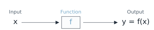
We now provide a more formal definition of a function and introduce several related concepts.

Definition: A Function

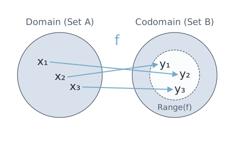
A function $f$ is a rule that assigns to each input $x\in A$ exactly one output $y\in B$. This relationship is often written as:

$$f:A\to B$$

In particular:

• The set $A$ is called the domain of the function. It contains all possible valid inputs.
• The set $B$ is called the codomain. It is the set into which all outputs are mapped.
• The range (also called the image) of the function is the set of actual outputs the function produces based on its domain. It is a subset of the codomain:

$$\mathrm{Range}(f)=\{f(x)\mid x\in A\}\subseteq B$$

A function always has a domain, which is the set of all inputs for which the function is defined. If no specific domain is stated for a function given by an equation, the default is typically the set of all real numbers that yield valid (usually real) outputs.

Functions are powerful tools for describing relationships between quantities. Many real-world scenarios can be modeled using functions, where one variable depends on another. In this context, it is also important to understand a function’s domain, codomain, and range, because these concepts clarify what kinds of inputs are valid, what types of outputs are expected, and what outputs actually occur.

Example: Temperature Over Time

The temperature at a given time of day can be expressed as a function of time. Suppose the temperature (in °C) follows the rule

$$T(t)=10+8\sin \left(\frac{\pi t}{12}\right)$$

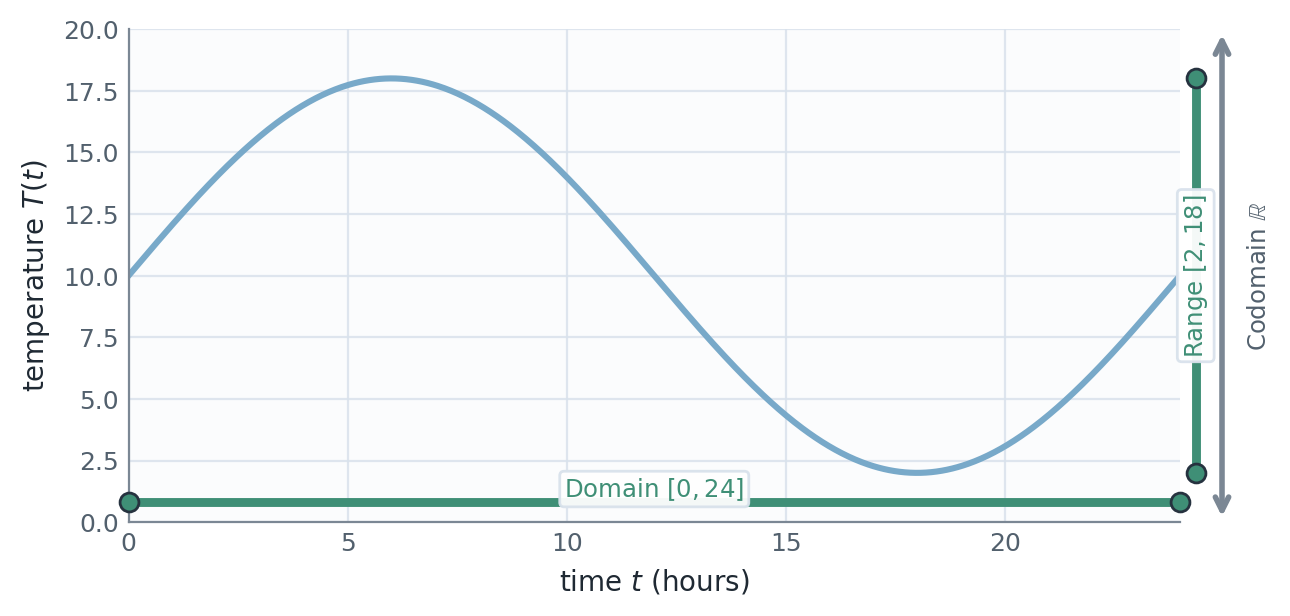
• Domain: $[0,24]$, because the model describes the time $t$ over a single day (in hours).
• Codomain: $\mathbb{R}$, since temperature values are real numbers.
• Range: $[2,18]$, since the sine term $\sin \left(\frac{\pi \cdot t}{12}\right)$ varies between $-1$ and $1$. This means $8\sin (\cdot )$ varies between $-8$ and $8$, and adding $10$ shifts the range to $[2,18]$.

Example: Distance Traveled at Constant Speed

If a car travels at a constant speed of 60 km/h, the distance traveled after $t$ hours is given by

$$D(t)=60t$$

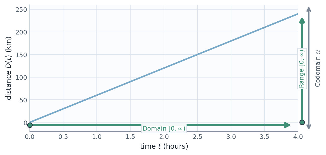
• Domain: $[0,\infty )$, because the time $t$ cannot be negative.
• Codomain: $\mathbb{R}$, since distances are expressed as real numbers.
• Range: $[0,\infty )$, because multiplying a non-negative $t$ by 60 produces a non-negative result. The distance is $D(0)=0$ at the start, and increases without bound as time increases.

Example: Customer Feedback from a Star Rating

A platform summarizes a customer's star rating as a feedback category. Let $r$ be the submitted rating and define

$$C:\{1,2,3,4,5\}\to \{\text{Negative},\text{Neutral},\text{Positive}\}$$

by

$$C(r)=\{\begin{array}{ll}\text{Negative},& r\in \{1,2\},\\ \text{Neutral},& r=3,\\ \text{Positive},& r\in \{4,5\}.\end{array}$$

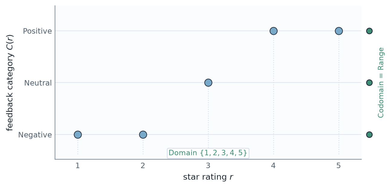
• Domain: $\{1,2,3,4,5\}$, the possible submitted star ratings.
• Codomain: $\{\text{Negative},\text{Neutral},\text{Positive}\}$, the declared feedback categories.
• Range: $\{\text{Negative},\text{Neutral},\text{Positive}\}$, because every declared category is attained by at least one rating.

Unlike the preceding examples, both the domain and codomain are discrete, and the outputs are categorical rather than numerical.

Representation Methods

Functions can be represented in several different ways, each offering different insights into the relationship they describe. Depending on the context, one representation may be more useful or informative than another.

To illustrate these representations, we will use a simplified example based on (synthetically generated) agriculture data. Let $f(x)$ denote the crop yield (in t/ha) as a function of fertilizer amount $x$ (in kg/ha). That is, we define:

$$f(x)=\text{yield corresponding to fertilizer amount }x$$

This example models a common real-world scenario where crop yield depends on the amount of fertilizer used.

Tables

A table is one of the most straightforward ways to represent a function. This form is especially useful when working with data collected through observation or measurement. Essentially, a table just lists specific input values and their corresponding output values.

Table 4.1. Selected input-output values for the crop-yield function.

In this table, each row shows a specific input value $x$ and the corresponding output value $f(x)$. Tables are useful for answering discrete queries, such as: "What is the crop yield if given 200 kg/ha fertilizer?".

They can also help identify general trends in the data, which leads us to the following definitions.

Definition: Increasing on an Interval

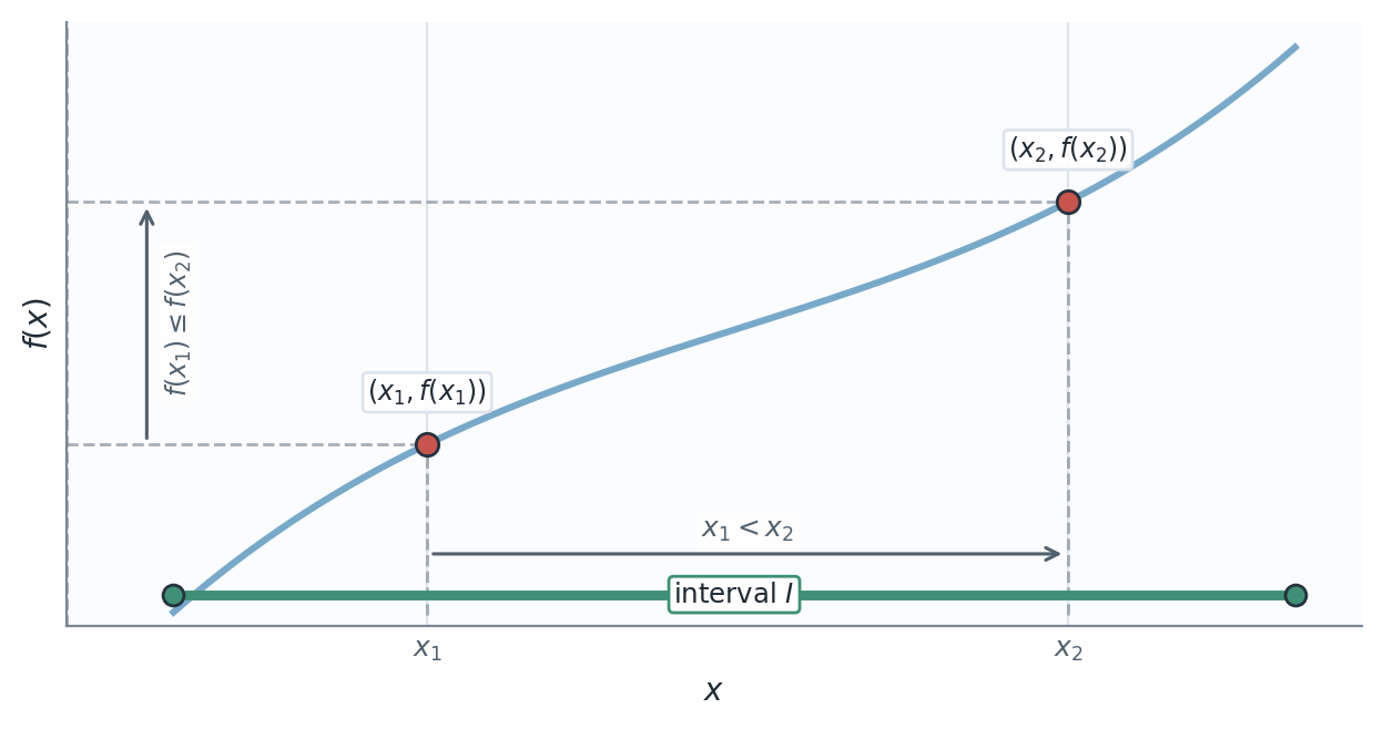
We say that a function $f$ is increasing on an interval $I$ if for all $x_1,x_2\in I$ it holds that

$$f(x_1)\le f(x_2),\text{when}{x}_1<x_2$$

The function $f$ is said to be strictly increasing (note the inequality) when

$$f(x_1)<f(x_2),\text{when}{x}_1<x_2$$

Definition: Decreasing on an Interval

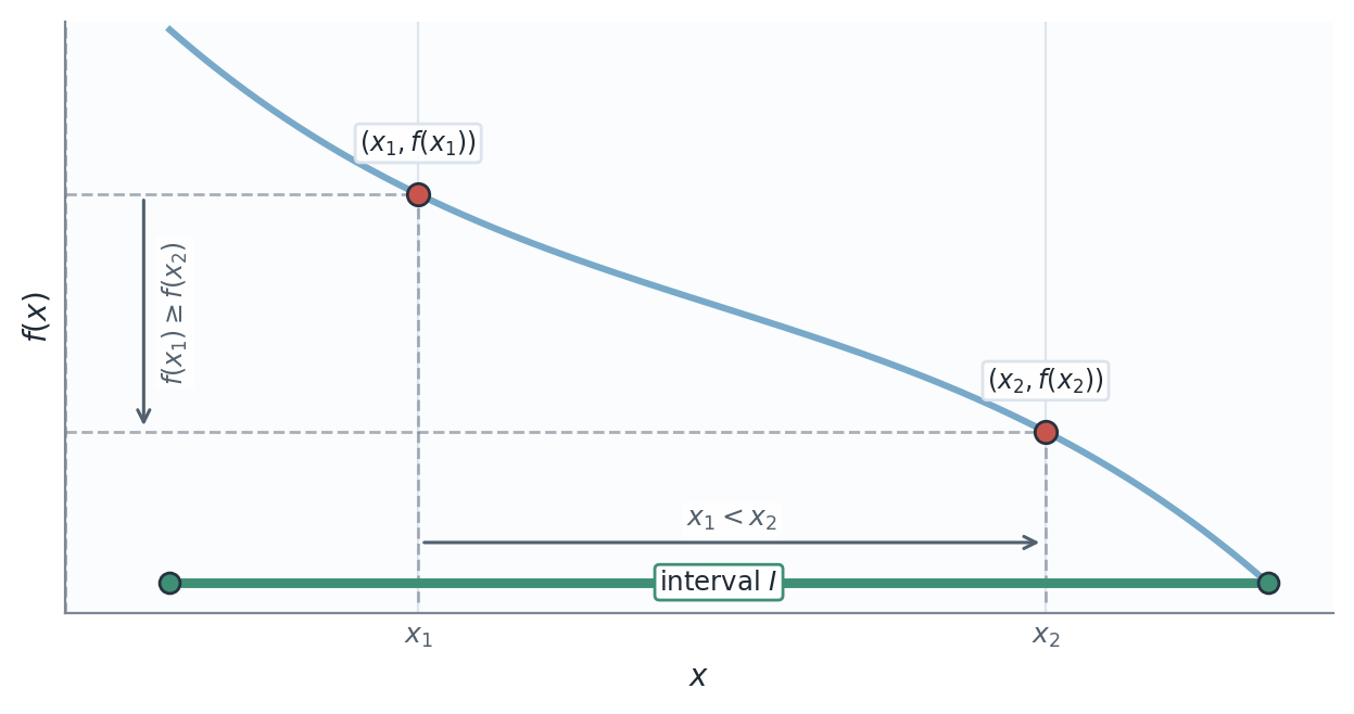
We say that a function $f$ is decreasing on an interval $I$ if for all $x_1,x_2\in I$ it holds that

$$f(x_1)\ge f(x_2),\text{when}{x}_1<x_2$$

The function $f$ is said to be strictly decreasing (note the inequality) when

$$f(x_1)>f(x_2),\text{when}{x}_1<x_2$$

By applying these definitions and inspecting the table, we can observe that the crop yield $f(x)$ increases as the fertilizer amount $x$ increases - up to a certain point - and then decreases. However, beyond this general behavior, it is difficult to tell much more. The table alone does not reveal whether the relationship is simply linear, or follows a more complex curve. In particular, it does not clearly convey the rate at which the crop yield increases or whether this rate changes over the domain. For such insights, a graphical or algebraic representation is usually more informative.

Graphs

A visual picture of a function can be provided in the form of a graph. The graph of a function is the set of points $(x,f(x))$ plotted in a coordinate plane, where $y=f(x)$ for all $x$ in the domain of $f$. Plotting data points from a table helps reveal the overall shape and behavior of the function, which may not be immediately apparent from a list of values alone.

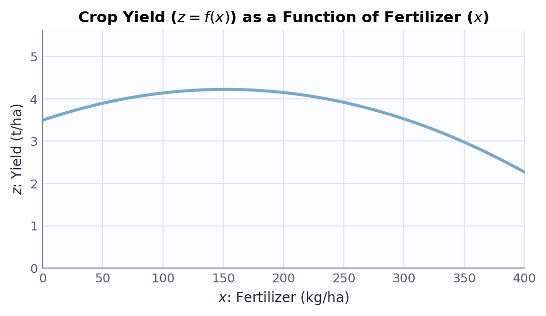
From this graph, we can observe that the function increases with fertilizer ($x$), to a point, but not linearly. The curve appears to flatten and then decrease more sharply, suggesting that the relationship between fertilizer ($x$) and yield ($f(x)$) is non-linear, possibly polynomial.

Algebraic Formulas

Often, we want more than just individual data points, we want a general rule that allows us to compute the output for any valid input. An algebraic formula provides a compact, symbolic way to describe the relationship between inputs and outputs.

The table and graph above were synthetically generated from the quadratic polynomial:

$$f(x)=-3.17042\cdot 10^{-5}\cdot x^2+0.00961968x+3.49418$$

The example is conceptual rather than a report of a particular experiment. In practice, a formula of this kind can be obtained from observed data by fitting a mathematical function to measurements. The resulting polynomial then approximates the relationship between fertilizer amount and crop yield, smoothing out random variation while preserving its overall pattern.

Having an algebraic representation allows us to carry out several useful analyses:

• Interpolation: Estimate values between known data points.
• Extrapolation: Predict behavior beyond the observed range, for instance, for very small or large fertilizer amounts ($x$).
• Equation solving: Find input values corresponding to specific outputs, for example solving $f(x)=4.0$ to determine the fertilizer amounts for which the model predicts a yield of 4.0 t/ha.

More broadly, models based on algebraic formulas let us describe and explore real-world phenomena: how quantities change together, where growth slows or reverses, and how one variable influences another. Such models form the foundation of mathematical analysis, offering insight into underlying behavior.

To describe these relationships effectively, we must choose a suitable type of function and fit it to the data. The displayed coefficients illustrate what a least-squares fit may produce; least squares is a method that finds a curve that closely matches observed data. Recognizing different classes of functions, such as linear, quadratic, cubic, or exponential, helps us select appropriate models and interpret the types of behavior they represent.

Basic Classes of Functions

Functions can be grouped into different classes based on their algebraic form. Each class has its own properties, domain and range, and characteristic graph shape. In this section, we focus on common basic function classes and describe their general forms (graphical) behavior.

Before exploring specific types, it is useful to note two important features that appear frequently in graphs of functions:

Table 4.2. Common graphical features of functions.

Polynomial Functions

Polynomial functions are smooth, continuous curves with no sharp corners or breaks. Their general behavior depends on the degree and the leading coefficient.

Definition: Polynomial Function

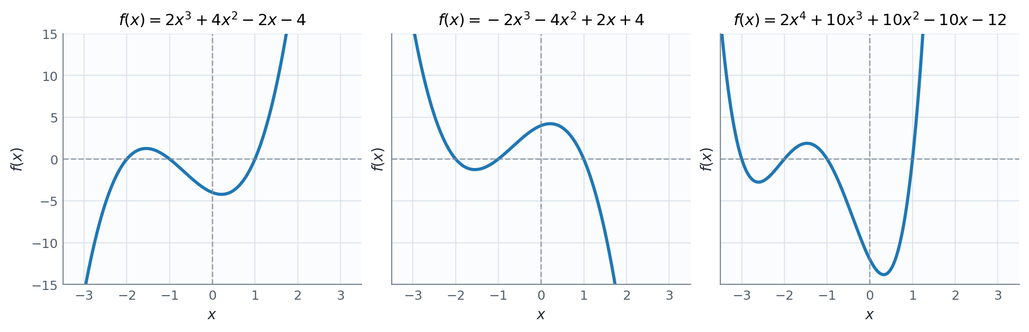
Nonzero polynomials belong to a broad class of functions that can be written in the general form:

$$f(x)=a_n{x}^n+a_{n-1}{x}^{n-1}+\cdots +a_{1}x+a_0$$

where:

• $n$ is a non-negative integer (the degree of the polynomial)
• $a_n,a_{n-1},\dots ,a_0$ are real constants
• $a_n\ne 0$

The zero polynomial $f(x)=0$ is also a polynomial, but its degree is left undefined in this course.

Key characteristics:

• Graph: smooth, continuous curve.
• Intercepts: A nonzero degree-$n$ polynomial has at most $n$ real $x$-intercepts; every polynomial has one point on the $y$-axis at $(0,a_0)$.
• Domain: $\mathbb{R}$.
• Range: Depends on the degree and coefficients.

Independently of its number of terms, a polynomial can also be classified by its degree, as described in the following.

Linear Functions

A linear function is a polynomial of degree $1$ and its graph is a straight line.

Definition: Linear Function

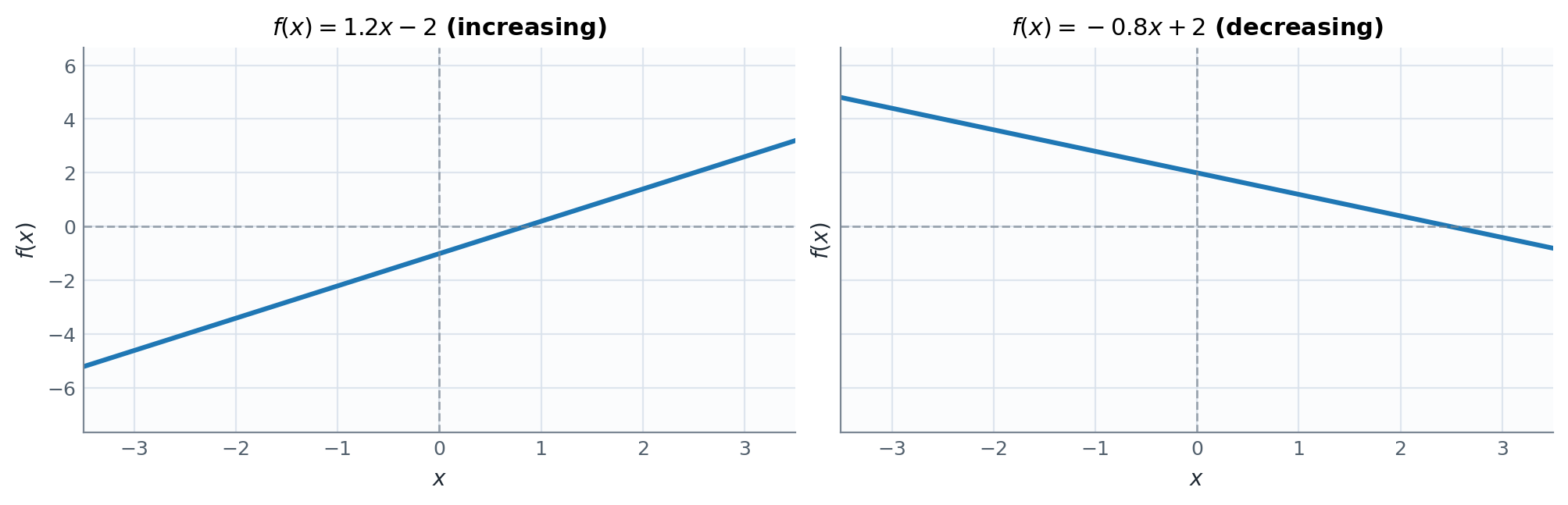
A linear function can be written in the general (slope-intercept) form:

$$f(x)=ax+b$$

where $a$ and $b$ are constants. If $a\ne 0$, it is a polynomial of degree $1$; if $a=0$, it simplifies to $f(x)=b$, which is a constant function (a polynomial of degree 0).

Key characteristics:

• Graph: A straight line with slope $a$.
  • If $a>0$ the function is increasing
  • If $a<0$ the function is decreasing
• Intercepts:
  • $y$-intercept at point $(0,b)$
  • If $a\ne 0$, one $x$-intercept at point $(-\frac{b}{a},0)$
• Domain: $\mathbb{R}$.
• Range: $\mathbb{R}$ if $a\ne 0$; if $a=0$, the range is the single-value set $\{b\}$.

One of the defining characteristics of a line is its slope. The slope describes how a line rises or falls as we move along the $x$-axis, i.e., in other words, it represents the rate of change in $y$ for each unit change in $x$.

The slope measures both the steepness and the direction of a line:

• If the slope is positive, the line points upward when moving from left to right
• If the slope is negative, the line points downward when moving from left to right
• If the slope is zero, the line is horizontal

To determine the slope numerically, we compare how much $y$ changes relative to $x$. This comparison gives us the ratio of the change in $y$ to the change in $x$, leading to the more formal definition below.

Now, let us explore how this definition relates to the formula of a linear function. Consider the function:

$$f(x)=ax+b$$

We already know that the graph of a linear function is a straight line. To find its slope, we can apply the definition above using any two points, i.e., $(x_1,y_1)$ and $(x_2,y_2)$, on the line. In particular, let us evaluate the function at two convenient points:

• When $x_1=0$, we have $y_1=f(0)=a\cdot 0+b=b$. This gives us the point: $$(x_1,y_1)=(0,b)$$
• When $x_2=1$, we have $y_2=f(1)=a\cdot 1+b=a+b$. This gives us the point: $$(x_2,y_2)=(1,a+b)$$

Therefore, substituting the points into the formula for the slope, the slope of this line is:

$$\begin{array}{rl}m& =\frac{y_2-y_1}{x_2-x_1}\\ & =\frac{(a+b)-b}{1-0}\\ & =\frac{a}{1}\\ & =a\end{array}$$

This shows that the coefficient $a$ in the function $f(x)=ax+b$ represents the slope of the line. Every function of this form describes a line with slope $a$ and $y$-intercept $b$; it is a degree-$1$ linear function when $a\ne 0$ and a constant function when $a=0$.

This relationship will be revisited in Chapter 10, where the concept of slope forms the basis for defining differentiation.

Quadratic Functions

A quadratic function is a polynomial of degree $2$; its graph is a parabola.

Definition: Quadratic Function

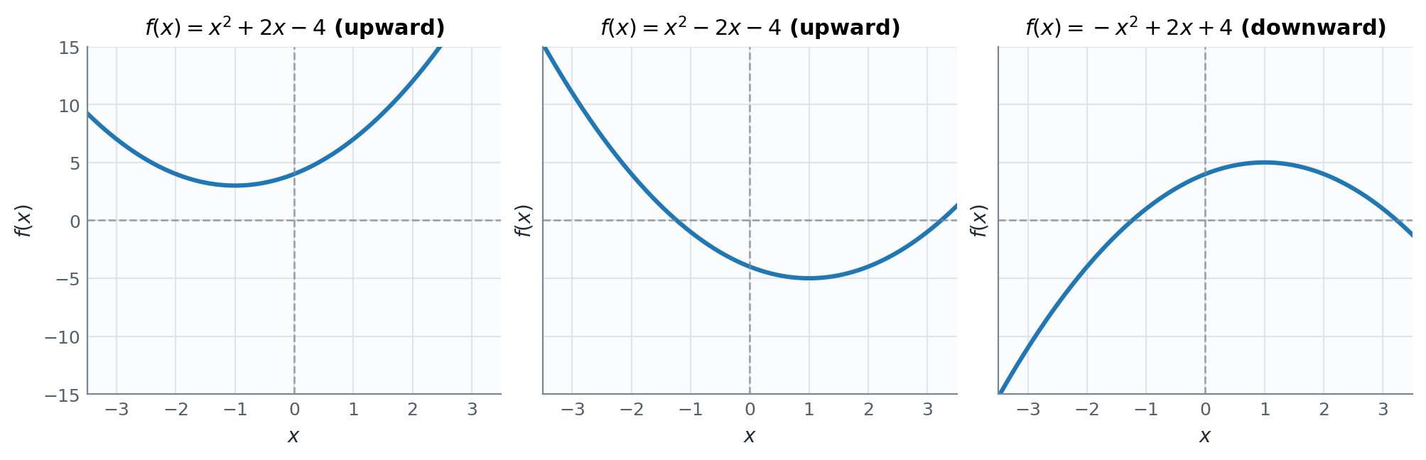
A quadratic function can be written in the general form:

$$f(x)=a{x}^2+bx+c$$

where $a\ne 0$.

Key characteristics:

• Graph: A parabola.
  • If $a>0$ the parabola opens upward
  • If $a<0$ the parabola opens downward
• Intercepts: Up to two $x$-intercepts, and exactly one $y$-intercept
• Turning Point (Vertex): The point $(x_v,y_v)$ where the graph changes direction.
  • If $a>0$, the vertex is the lowest point, so $y_v=y_{\min }$
  • If $a<0$, the vertex is the highest point, so $y_v=y_{\max }$
• Domain: $\mathbb{R}$.
• Range:
  • If $a>0$ it is $[y_{\min },\infty )$
  • If $a<0$ it is $(-\infty ,y_{\max }]$

Exponential Functions

Exponential functions have a constant base raised to a variable exponent.

Definition: Exponential Function

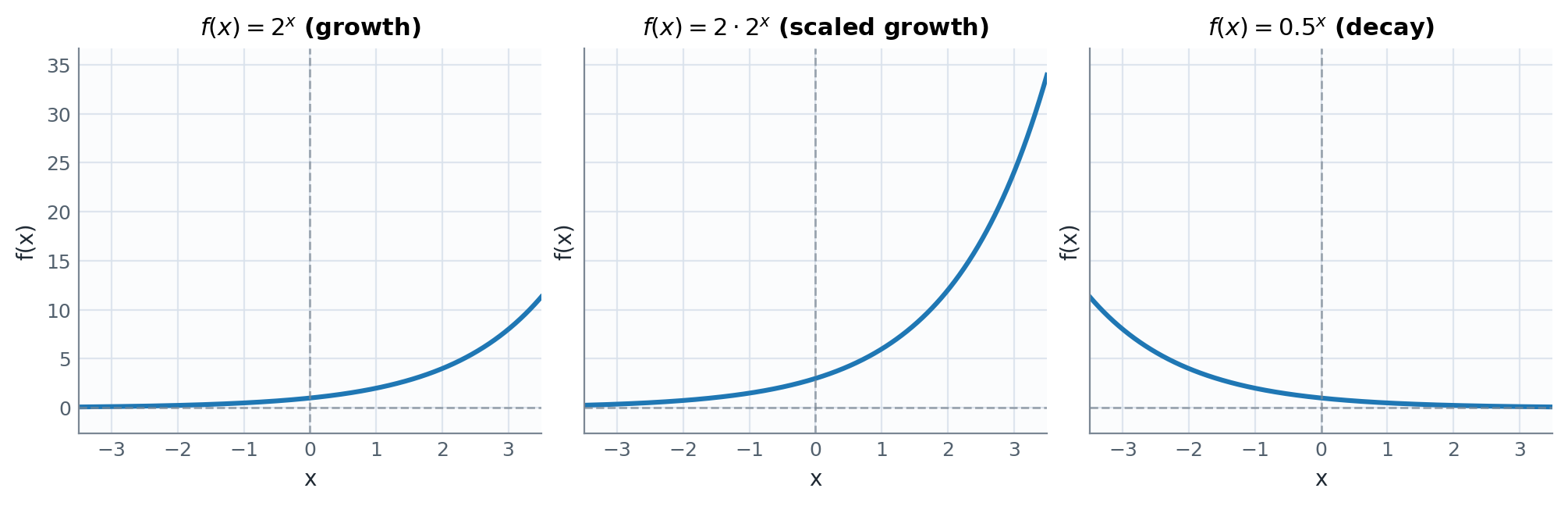
An exponential function can be written in the general form:

$$f(x)=a{b}^x$$

where $a\ne 0$, $b>0$, and $b\ne 1$.

The magnitude $|a|$ is the vertical scale factor relative to $b^x$; if $a<0$, the graph is also reflected across the $x$-axis.

Key characteristics:

• Graph:
  • If $a>0$ and $b>1$, the graph is increasing (growth)
  • If $a>0$ and $0<b<1$, the graph is decreasing (decay)
  • If $a<0$, these directions are reversed because the graph is reflected across the $x$-axis
• Asymptote: Horizontal at $y=0$.
• Domain: $\mathbb{R}$.
• Range: $(0,\infty )$ if $a>0$, and $(-\infty ,0)$ if $a<0$.

Logarithmic Function

Logarithmic and exponential functions have an important relationship: each operation undoes the other. Applying a logarithm after exponentiation returns the original exponent,

$${\log }_b\left(b^y\right)=y,$$

while exponentiating after taking a logarithm returns the original positive number,

$$b^{{\log }_b(x)}=x.$$

Together, these two relationships can be written compactly as

$$y={\log }_b(x)\iff b^y=x,$$

where $x>0$, $y\in \mathbb{R}$, $b>0$, and $b\ne 1$.

The relationship works in both directions. Knowing either equation gives us the other. The idea of undoing one operation with another is central to equation solving and will be studied further in Chapter 7.

Definition: Logarithmic Function

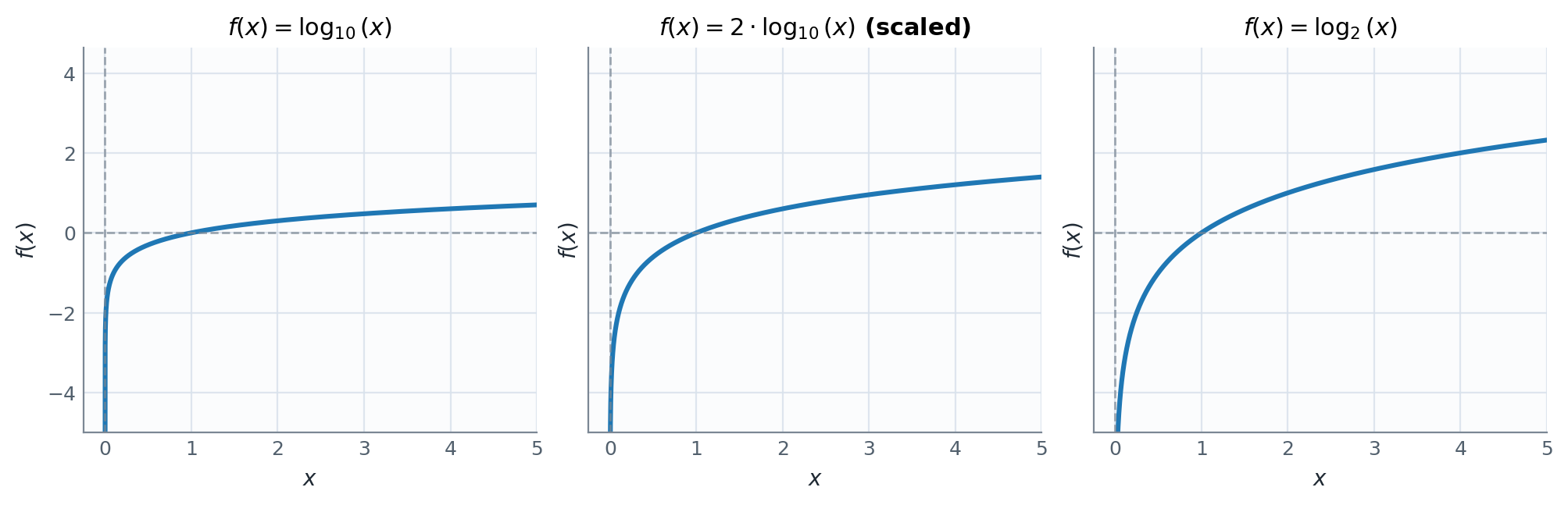
A logarithmic function can be written in the general form:

$$f(x)=a\cdot {\log }_b(x)$$

where $a\ne 0$, $b>0$, and $b\ne 1$.

The magnitude $|a|$ is the vertical scale factor relative to ${\log }_b(x)$; if $a<0$, the graph is also reflected across the $x$-axis.

Key characteristics:

• Graph:
  • Passes through $(1,0)$ for every $a\ne 0$
  • If $a>0$, it is increasing for $b>1$ and decreasing for $0<b<1$; a negative $a$ reverses these directions
  • Is unbounded above and below across its domain
• Asymptote: Vertical at $x=0$.
• Domain: $(0,\infty )$.
• Range: $\mathbb{R}$.

Piecewise Functions

Not all functions can be described by a single formula. In some cases, different rules apply to different parts of the domain. Such functions are called piecewise functions, or piecewise-defined functions.

Example: Piecewise Function with Two Rules

The graph below shows how two different formulas can describe one function on different parts of its domain.

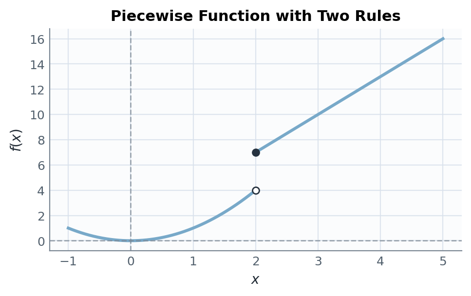
Consider the function defined by

$$f(x)=\{\begin{array}{ll}3x+1,& \text{if }x\ge 2,\\ x^2,& \text{if }x<2.\end{array}$$

To evaluate a piecewise function, first determine which part of the domain the input belongs to, and then apply the corresponding rule. For instance:

• For $x=5$, since $5\ge 2$, use function $3x+1$: $$f(5)=3\cdot 5+1=16$$
• For $x=-1$, since $-1<2$, use function $x^2$: $$f(-1)=(-1{)}^2=1$$

Example: Absolute Value Function

The absolute value function is a familiar example where the rule changes at zero.

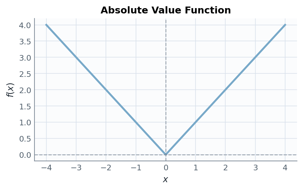
The absolute value function, denoted by $f(x)=|x|$, can be expressed as a piecewise function:

$$f(x)=\{\begin{array}{ll}x,& \text{if }x\ge 0,\\ -x,& \text{if }x<0.\end{array}$$

Here, positive inputs are unchanged, while negative inputs are reflected across the $x$-axis, ensuring that $f(x)$ is always non-negative.

Example: ReLU Function

Another common piecewise example comes from machine learning, where negative inputs are clipped to zero.

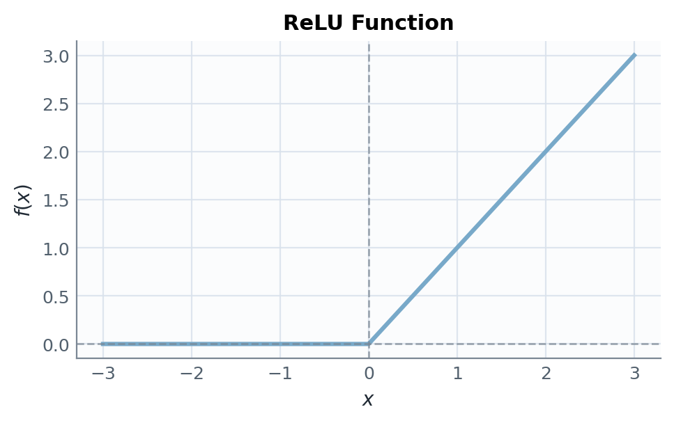
The Rectified Linear Unit (ReLU) is a commonly used activation function in neural networks. It can be expressed as a piecewise function:

$$f(x)=\{\begin{array}{ll}x,& \text{if }x>0,\\ 0,& \text{if }x\le 0.\end{array}$$

The ReLU function outputs the input value itself when it is positive, and zero otherwise. This simple non-linear behavior introduces nonlinearity into neural networks, which is an essential property that allows them to learn complex patterns and relationships in data.