Chapter 5: Equation Solving

Equations express the equality of two expressions and are essential tools for modeling and solving real-world problems. While a function describes the relationship between variables, solving an equation means finding the variable values that make the equality true. This section focuses on linear and quadratic equations, highlighting how their solutions, i.e., the roots, connect algebraic methods with geometric interpretation. We will also extend these ideas to equation-solving for other basic classes of functions introduced earlier.

Earlier, we described functions and particular points associated with the graph of a function that are typically of interest due to what they represent. We described $x$ - and $y$ -intercepts, where:

The $x$ -intercepts are the points at which the output value is zero.
The $y$ -intercept is the point at which the function has an input value of zero.

Analytically, these points can be found by solving:

$x$ -intercepts: solve $f (x) = 0$
$y$ -intercept: solve $f (0) = y$

Both of these tasks are examples of equation solving, i.e., we set a function equal to a specific value (often zero) and find the corresponding input(s). The process of solving an equation, therefore, has both an algebraic side (manipulating numbers and symbols to isolate the variable) and a geometric side (finding where a graph meets a horizontal or vertical axis).

Concept: Solving an Equation

Using algebraic properties, we "isolate" a particular variable on one side of the equality sign so that we obtain a solution in the form:

$x = "stuff"$

where "stuff" can be an expression containing numbers, constants, other variables, and mathematical operators such as addition, subtraction, multiplication, division, square root, and the like.

Solutions to Equations as Roots

The concept of a root is central to solving many types of equations, fundamentally linking algebraic solutions to graphical interpretations.

Definition: Root (or Zero) of a Function

A root of a function $f (x)$ is a point $x$ such that $f (x) = 0$ .

Graphically, these are the points where the function's graph intersects the $x$ -axis (i.e., a root is synonymous with the function's $x$ -intercepts).

Any equation of the form $f (x) = g (x)$ can be transformed into the problem of finding the roots of a new function:

$h (x) = f (x) - g (x)$

This means that solving for the equality of two functions is equivalent to finding the $x$ -intercepts of their difference.

Solving Linear Equations

In this section, we illustrate the equation-solving process for the case where the resulting function $h (x) = f (x) - g (x)$ is linear. In such cases, solving $f (x) = g (x)$ is equivalent to finding the root of the linear function $h (x)$ .

Example 1: Roots of a Linear Function

*Left: Graphs of the given functions $f$ and $g$ . Right: Solving $f (x) = g (x)$ as a root-finding problem for the resulting linear function $h (x) = f (x) - g (x)$ .*

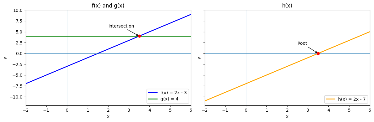
Consider the functions:

$f (x) = 2 x - 3 and g (x) = 4$

Here, $f (x)$ is linear and $g (x)$ is a constant function.

Finding the intersection of the graphs means determining $x$ such that:

$f (x) = g (x) \Leftrightarrow 2 x - 3 = 4$

We can convert this into a root-finding problem by moving all terms to one side, expressing the equation in the standard form $h (x) = 0$ :

$\Leftrightarrow \Leftrightarrow f (x) - g (x) 2 x - 3 - 4 2 x - 7 = 0 = 0 = 0$

Here, the left-hand side can be regarded as a new function $h (x) = 2 x - 7$ . Finding its root is equivalent to solving the original equation:

$\Leftrightarrow \Leftrightarrow \Leftrightarrow \Leftrightarrow \Leftrightarrow h (x) 2 x - 7 2 x \frac{2 x}{2} x x = 0 = 0 = 7 = \frac{7}{2} = \frac{7}{2} = 3.5$

The solution $x = 3.5$ represents the point where the graphs of $f (x)$ and $g (x)$ intersect. In terms of the root-finding approach, this is the zero of $h (x)$ , i.e., the value of $x$ for which $h (x)$ crosses the $x$ -axis.

Solving Quadratic Equations

In this section, we illustrate the equation-solving process for the case where the resulting difference $h (x) = f (x) - g (x)$ is quadratic. In such cases, solving $f (x) = g (x)$ is equivalent to finding the root of the quadratic function $h (x)$ .

Example: Roots of a Quadratic Function

*Left: Graphs of the given functions $f$ and $g$ . Right: Solving $f (x) = g (x)$ as a root-finding problem for the resulting quadratic function $h (x) = f (x) - g (x)$ .*

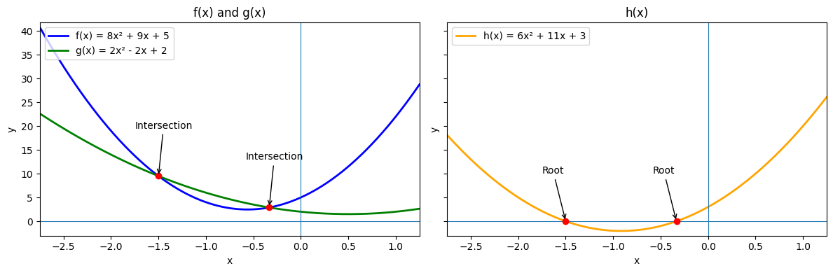
Consider the functions:

$f (x) = 8 x^{2} + 9 x + 5 and g (x) = 2 x^{2} - 2 x + 2$

Here, $f (x)$ and $g (x)$ are both quadratic.

Finding the intersection of the graphs means determining $x$ such that:

$f (x) = g (x) \Leftrightarrow 8 x^{2} + 9 x + 5 = 2 x^{2} - 2 x + 2$

We convert this to a root-finding problem by moving everything to one side:

$\Leftrightarrow \Leftrightarrow \Leftrightarrow f (x) - g (x) (8 x^{2} + 9 x + 5) - (2 x^{2} - 2 x + 2) 8 x^{2} + 9 x + 5 - 2 x^{2} + 2 x - 2 6 x^{2} + 11 x + 3 = 0 = 0 = 0 = 0$

At this stage, we have reduced the problem to solving a quadratic equation:

$h (x) = 6 x^{2} + 11 x + 3 = 0$

There are two standard ways to find its roots:

By factoring the quadratic expression into a product of two linear factors.
By applying the quadratic formula, which works even when factoring is not straightforward.

In the examples that follows, we will illustrate both approaches, using the same function $h (x)$ .

Solving Via Factorization

Factoring a quadratic expression means expressing it as a product of two linear factors. If this is possible, the zero product property can be applied:

$a \cdot b = 0 \Rightarrow a = 0 or b = 0$

This allows us to solve a quadratic equation by setting each factor equal to zero.

Example: Solving by Factorization

We are given the quadratic polynomial

$h (x) = 6 x^{2} + 11 + 3$

and want to factorize it using the grouping method, which we learned about in the previous Chapter 4.

The expression contains three terms, but the grouping method requires four. Thus, the first step is to rewrite the trinomial as a four-term polynomial. We can do this using Algorithm 1 from Chapter 4.

Step 1:: Identify coefficients:

$a = 6$ is the coefficient of the higest-order term $x^{2}$
$b = 11$ is the coefficient of the second-highest-order term $x$
$c = 3$ is the constant term

Step 2: Find two integers $m$ , $n$ such that

$m \cdot n = a \cdot c = 6 \cdot 3 = 18$
$m + n = b = 11$

Choosing $m = 9$ and $n = 2$ satisfies these conditions since $m \cdot n = 18$ and $m + n = 11$ .

Step 3: Rewrite the middle term using $m$ and $n$ : $6 x^{2} + 11 x + 3 = 6 x^{2} + m x 9 x + n x 2 x + 3$

Now we can apply the grouping method as described in Algorithm 2.

Step 1: Group the terms into pairs:

$(6 x^{2} + 9 x) + (2 x + 3)$

Step 2: Factor out the greatest common factor (GCF) from each group:

$3 x (2 x + 3) + 1 (2 x + 3)$

Step 3: A Common binomial factor appears:

$(2 x + 3) (3 x + 1) = 0.$

Finally, we can now apply the zero product property to solve for $x$ :

$2 x + 3 = 0 \Rightarrow x = - \frac{3}{2} and 3 x + 1 = 0 \Rightarrow x = - \frac{1}{3}$

Solving Via The Quadratic Formula

Another way to find the roots of $h (x)$ is to apply the quadratic formula.

Definition: The Quadratic Formula

Consider the quadratic equation:

$a x^{2} + b x + c = 0$

where $a \neq = 0$ . The solutions of this equation is given by the quadratic formula:

$x = \frac{- b \pm b ^{2} - 4 a c}{2 a}$

The discriminant $Δ = b^{2} - 4 a c$ determines the number of real solutions:

If $Δ > 0$ : two distinct real solutions.
If $Δ = 0$ : one real (repeated) solution.
If $Δ < 0$ : no real solutions.

Note: the $\pm$ symbol in the formula above means that we consider the expression both when the square root positive and negative.

Example: The Quadratic Formula

To solve the quardratic equation

$h (x) = 0 \Leftrightarrow 6 x^{2} + 11 + 3 = 0$

we set $a = 6$ , $b = 11$ , and $c = 3$ in the formula:

$x = \frac{- b \pm b ^{2} - 4 a c}{2 a} = \frac{- 11 \pm 1 1 ^{2} - 4 \cdot 6 \cdot 3}{2 \cdot 6} = \frac{- 11 \pm 121 - 72}{12} = \frac{- 11 \pm 49}{12}$

Hence, we get:

$x = \frac{- 11 + 7}{12} = - \frac{4}{12} = - \frac{1}{3} or x = \frac{- 11 - 7}{12} = - \frac{18}{12} = - \frac{3}{2}$

These match the solutions obtained by factoring.

Factorized Form and Roots of a Polynomial

Just as quadratic equations can be expressed in factorized form as

$f (x) = a (x - r_{1}) (x - r_{2})$

higher-order polynomials can likewise be written as a product of linear factors. This leads us to the following definition.

Definition: Factorized Form of a Polynomial

A polynomial function $f (x)$ of degree $n$ can be expressed as

$f (x) = a (x - r_{1}) (x - r_{2}) \dots (x - r_{n}),$

where $a$ is the leading coefficient and each $r_{i}$ is a root (or zero) satisfying $f (r_{i}) = 0$ .

This form reveals several geometric features of the polynomial:

The number of factors equals the degree of the polynomial
Each root $r_{i}$ corresponds to an $x$ -intercept of the graph
The coefficient $a$ determines the vertical stretch and orientation of the curve. For example, changing its sign reflects the graph across the $x$ -axis.

The following examples illustrate how these properties appear graphically.

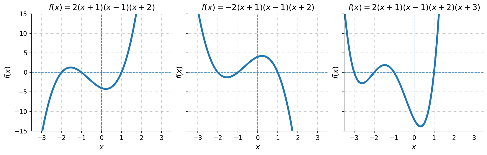
Examples: Factorized Form of a Polynomial

*Polynomials in factorized form. Each root $(x = r_{i})$ corresponds to an $x$ -intercept where $f (x) = 0$ .*

Consider the first polynomial in the plot:

$f (x) = 2 (x + 1) (x - 1) (x + 2)$

This function has three linear factors, so the polynomial is of degree three. The zeros, listed in the order they appear in the algebraic expression, are $x = - 1$ , $x = 1$ , and $x = - 2$ . At each of these points, one factor becomes zero, defining an $x$ -intercept where the graph meets the $x$ -axis.

Now look at the second polynomial in the plot:

$f (x) = - 2 (x + 1) (x - 1) (x + 2)$

The only difference is the sign of the leading coefficient. Changing it from $2$ to $- 2$ reflects the entire graph across the $x$ -axis, while the zeros remain in the same order and at the same positions.

Finally, consider the third polynomial in the plot:

$f (x) = 2 (x + 1) (x - 1) (x + 2) (x + 3)$

Here we have four linear factors, so the polynomial is of degree four. The zeros, again listed in the order of the factors, are $x = - 1$ , $x = 1$ , $x = - 2$ , and $x = - 3$ . As before, each root defines an $x$ -intercept where the graph meets the $x$ -axis.

The Sign and Behavior of a Function Around Its Roots

Finding the roots of a function does more than just tell us where it intercepts the $x$ -axis: It also reveals where the function takes on positive or negative values.

By analyzing the sign of $f (x)$ between its roots, we can determine on which intervals the function lies above or below the $x$ -axis, and thus describe its overall behavior.

The concepts of a function being Increasing on an Interval and Decreasing on an Interval further describe how the function behaves within those intervals, i.e., whether it rises or falls as $x$ changes.

These ideas are closely related: once the roots are known and the sign of $f (x)$ is determined, examining whether the function is increasing or decreasing helps us describe its overall shape and how it varies. Together, they provide a more complete picture of a function’s behavior, even without graphing it.

Definition: Positive and Negative Intervals

Let $f (x)$ be a real-valued function. We say that:

$f (x)$ is positive on an interval if $f (x) > 0$ for all $x$ in that interval.
$f (x)$ is negative on an interval if $f (x) < 0$ for all $x$ in that interval.

Graphically, this corresponds to whether the graph of the function lies above (positive) or below (negative) the $x$ -axis.

Because the sign of a function can only change at its roots, we can use the roots to divide the real line into intervals and then determine the sign of $f (x)$ within each one.

Example: Determining the Function Sign

For our quadratic function $h (x) = 6 x^{2} + 11 x + 3$ , we found earlier, that the roots are:

$x = - \frac{3}{2} and x = - \frac{1}{3} .$

These roots divide the real line into three intervals:

$(- \infty, - \frac{3}{2}), (- \frac{3}{2}, - \frac{1}{3}), (- \frac{1}{3}, \infty) .$

By testing a single point in each interval (for instance, $x = - 2, - 1, 0$ ), we find:

Interval	Test Value	Sign of $h (x)$	Behavior
$(- \infty, - \frac{3}{2})$	$x = - 2$	$h (- 2) = - 5 > 0$	$h (x)$ is positive
$(- \frac{3}{2}, - \frac{1}{3})$	$x = - 1$	$h (- 1) = - 2 < 0$	$h (x)$ is negative
$(- \frac{1}{3}, \infty)$	$x = 0$	$h (- 0) = - 3 > 0$	$h (x)$ is positive

Inverse Functions

When solving an equation of the form:

$f (x) = k$

we often want a general way to determine the input $x$ for any output value $k$ (in $f$ 's codomain). For some functions, it is possible to find another function that "reverses" the mapping performed by $f$ . This reversing function is called the inverse function.

Definition: Inverse of a Function

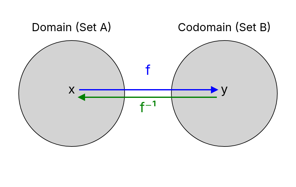
Let $f : A \to B$ be a function. An inverse function $f^{- 1} : B \to A$ satisfies:

$f^{- 1} (f (x)) = x and f (f^{- 1} (y)) = y$

for all $x \in A$ and $y \in B$ . This means that applying $f$ followed by $f^{- 1}$ (or vice versa) brings us back to the original value.

The inverse function essentially allows us to solve equations by applying $f^{- 1}$ to both sides:

$f (x) = y \Rightarrow \Leftrightarrow f^{- 1} (f (x)) x = f^{- 1} (y) = f^{- 1} (y)$

However, not every function has an inverse. Understanding when an inverse exists is thus essential.

Warning: Existence Conditions and Common Mistakes

A function $f$ has an inverse only if it is bijective, that is:
- Injective (one-to-one): no two inputs give the same output.
- Surjective (onto): every element of the codomain is produced by some input.
Otherwise, the mapping cannot be uniquely reversed.
The notation $f^{- 1}$ represents the inverse function, not the reciprocal: $f^{- 1} (x) \neq = \frac{1}{f ( x )} .$ The superscript $- 1$ indicates reversal of the mapping, not exponentiation.

Definition: Identity Property of Inverses

The composition of a function and its inverse returns the identity function on the respective domains:

$f \circ f^{- 1} = id_{B}, f^{- 1} \circ f = id_{A} .$

That is, the inverse of a function $f$ reverses the domain and codomain of $f$ . Graphically, the inverse corresponds to reflecting the graph of $f$ across the line $y = x$ .

Example: Finding an Inverse Function

Suppose $f : A \to B$ is defined by

$f (x) = 3 x + 5$

To find $f^{- 1}$ , solve for $x$ in terms of $y$ :

$y = 3 x + 5 \Leftrightarrow \Leftrightarrow y - 5 \frac{y - 5}{3} = 3 x = x$

This expression tells us how to recover $x$ from a given output $y$ , so:

$f^{- 1} (y) = \frac{y - 5}{3}$

Now, suppose we want to solve the equation:

$f (x) = 14$

To determine for which value of $x$ the function $f (x)$ is euqal to $14$ , we need to isolate $x$ on one side of the equality sign. Since we have already found the inverse of the function we can achieve this by applying $f^{- 1}$ to both sides:

$f^{- 1} (f (x)) = f^{- 1} (14)$

Since $f^{- 1}$ reverses the action of $f$ , the left-hand side simplifies to $x$ :

$x = \frac{14 - 5}{3} = 3$

In general, this is the reason for applying $f^{- 1}$ to both sides: it "undoes" $f$ on the side of the equality containing $x$ , essentially leaving $x$ alone.

Example: Verifying an Inverse Function

Consider the function in the earlier example, along with its inverse:

$f (x) = 3 x + 5 and f^{- 1} (y) = \frac{y - 5}{3}$

We can always check our work, by verifying the inverse properties, that is:

$f^{- 1} (f (x)) = x and f (f^{- 1} (y)) = y .$

Doing so, we indeed see that:

$f^{- 1} (f (x)) = f^{- 1} (3 x + 5) = \frac{( 3 x + 5 ) - 5}{3} = x$

Moreover, we see that:

$f (f^{- 1} (y)) = 3 (\frac{y - 5}{3}) + 5 = y$

Thus, $f (x) = 3 x + 5$ and $f^{- 1} (y) = \frac{y - 5}{3}$ are true inverses: each "undoes" the other's operation. In particular, $f$ multiplies by $3$ and adds $5$ , while $f^{- 1}$ subtracts $5$ and divides by $3$ , reversing the steps in the opposite order.

Common Inverses

Each of the examples given below show frequently used function-inverse pairs with their domains and ranges.

Example: Linear Shift

Example: Linear Scaling

Example: Power and Root Functions

Logarithm Rules

Since logarithms are inverse functions of exponentials, each rule in the table above can be derived directly from the exponent rules defined in Chapter 5.

Example: ...

Function $f (x)$	Inverse $f^{- 1} (x)$	Domain of $f$	Range of $f$
$f (x) = x + a$	$f^{- 1} (x) = x - a$	$R$	$R$
$f (x) = x - a$	$f^{- 1} (x) = x + a$	$R$	$R$
$f (x) = k x$ , $k \neq = 0$	$f^{- 1} (x) = \frac{x}{k}$	$R$	$R$
$f (x) = \frac{x}{k}$ , $k \neq = 0$	$f^{- 1} (x) = k x$	$R$	$R$
$f (x) = x^{n}$ , $n$ odd	$f^{- 1} (x) = n x$	$R$	$R$
$f (x) = x^{n}$ , $n$ even	$f^{- 1} (x) = n x$ (principal root)	$[0, \infty)$	$[0, \infty)$
$f (x) = e^{x}$	$f^{- 1} (x) = ln (x)$	$R$	$(0, \infty)$
$f (x) = a^{x}$ , $a > 0, a \neq = 1$	$f^{- 1} (x) = lo g_{a} (x)$	$R$	$(0, \infty)$
$f (x) = ln (x)$	$f^{- 1} (x) = e^{x}$	$(0, \infty)$	$R$
$f (x) = lo g_{a} (x)$ , $a > 0, a \neq = 1$	$f^{- 1} (x) = a^{x}$	$(0, \infty)$	$R$

Logarithm Rules

For $a > 0$ , $b > 0$ , $n \in R$ , and $a, b \neq = 1$ , the most important rules are given in the following table.

Rule	Formula	Description
Product Rule	$lo g_{b} (x \cdot y) = lo g_{b} (x) + lo g_{b} (y)$	The logarithm of a product equals the sum of the logarithms.
Quotient Rule	$lo g_{b} (\frac{x}{y}) = lo g_{b} (x) - lo g_{b} (y)$	The logarithm of a quotient equals the difference of the logarithms.
Power Rule	$lo g_{b} (x^{n}) = n \cdot lo g_{b} (x)$	A power in the argument becomes a multiplier in front of the logarithm.
Logarithm of 1	$lo g_{b} (1) = 0$	Any base raised to the power 0 equals 1.
Logarithm of the Base	$lo g_{b} (b) = 1$	Any base raised to the power 1 equals itself.
Inverse Property	$b^{l o g_{b} (x)} = x$	Exponential and logarithmic functions cancel each other.
Natural Log of $e$	$ln (e) = 1$	Since $ln (x)$ means $lo g_{e} (x)$ .
Change of Base	$lo g_{b} (x) = \frac{l o g _{k} ( x )}{l o g _{k} ( b )}$	Converts a logarithm from one base to another.

Note: The natural logarithm $ln (x)$ is simply $lo g_{e} (x)$ , where $e \approx 2.71828$ is Euler's number. All these rules work the same way for $ln$ as for $lo g_{b}$ for any base $b > 0$ , $b \neq = 1$ .

Since logarithms are inverse functions of exponentials, each rule in the table above can be derived directly from the exponent rules defined in Chapter 5.

Solving Non-Linear Equations

Many equations in mathematics involve non-linear functions such as exponentials and logarithms. The solving principles remain the same: we transform the equation into an equivalent one where the variable of interest is isolated, checking that the solution satisfies any domain restrictions.

A common strategy for solving these equations is to undo an operation using its inverse. In this context, we can make direct use of the inverse function pairs introduced earlier. In particular, when the variable appears in an exponent, we apply a logarithm to both sides, and when it appears inside a logarithm, we apply an exponential.

Example: Solving an Exponential Equation

Let us solve the equation $e^{2 x + 1} = w$ , $w > 0$ for $x$ .

$\Leftrightarrow \Leftrightarrow \Leftrightarrow e^{2 x + 1} ln (e^{2 x + 1}) 2 x + 1 x = w = ln (w) = ln (w) = \frac{1}{2} (ln (w) - 1)$

Example: Solving a Logarithmic Equation

Solve the equation $ln (x^{2} - 10) = 6$ for $x$ . Assume that $x^{2} > 10$ , as the logarithm otherwise is not defined. We obtain:

$\Leftrightarrow \Leftrightarrow \Leftrightarrow \Leftrightarrow ln (x^{2} - 10) e^{l n (x^{2} - 10)} x^{2} - 10 x^{2} x = 6 = e^{6} = e^{6} = e^{6} + 10 = \pm e^{6} + 10$

Determining Whether a Relation is a Function

Graphically

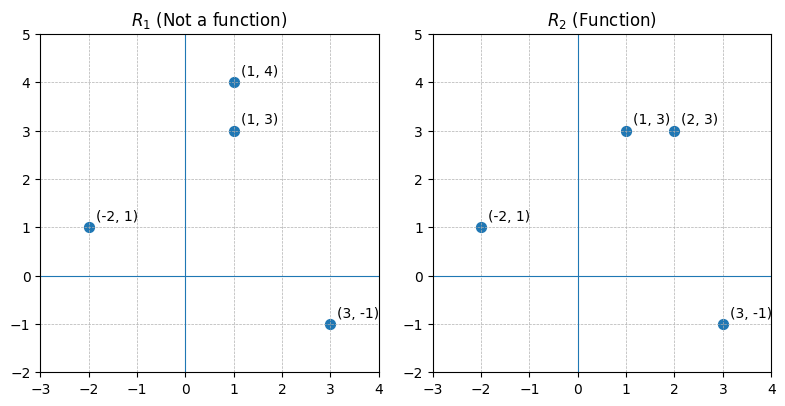
A relation in which each $x$ -coordinate is matched with exactly one $y$ -coordinate is said to describe $y$ as a function of $x$ . This also means that, if the same $x$ -coordinate is associated with two different $y$ -coordinates, then the relation is not a function.

Example: Checking Functional Relations

Which of the following relations descbribe $y$ as a function of $x$ ?

$R_{1} = {(- 2, 1), (1, 3), (1, 4), (3, - 1)}$
$R_{2} = {(- 2, 1), (1, 3), (2, 3), (3, - 1)}$

Inspecting the points of $R_{1}$ reveals that the $x$ -coordinate $1$ is matched with two different $y$ -coordinates: Namely $y = 3$ and $y = 4$ . Hence in $R_{1}$ , y is not a function of $x$ . On the other hand, every $x$ -coordinate in $R_{2}$ occurs only once which means each $x$ -coordinate has only one corresponding $y$ -coordinate. So, $R_{2}$ does represent $y$ as a function of $x$ . We can verify this graphically as well:

$R_{1} $ fails (same $x$ with different $y$ ); $R_{2}$ passes (each $x$ has one $y$ )

The Vertical Line Test

More generally, this also leads to the vertical line test, which is a quick graphical method to decide whether a relation is a function.

Definition: Vertical Line Test

Polynomial (function) passes the test; circle (not a function) fails. Intersection points are marked.

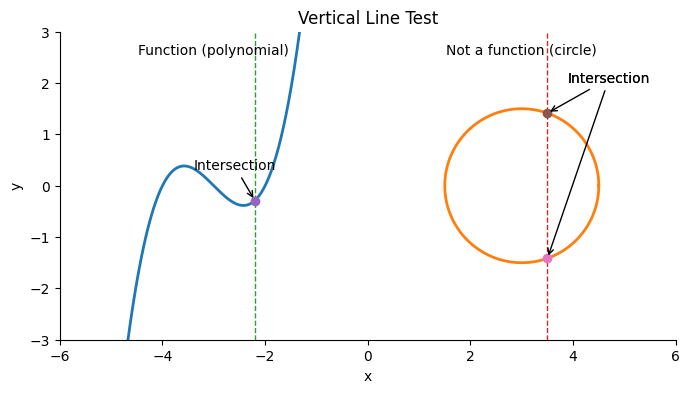
A relation is a function if and only if every vertical line intersects its graph at most once.

If a vertical line intersects more than once, the relation assigns more than one output to the same input thus violating the definition of a function.

It is important to note that equations can describe valid relationships—like the shape of a circle—but do not define a function. Recognizing this helps us understand both the limits of function notation and the situations where we need use other representations (such as parametric or implicit forms).

Algebraically

We can also check whether an equation defines a function by solving for one variable in terms of the other. If solving produces more than one output value for the same input, then the relation is not a function.

Example: Equation That Is Not a Function

Does the equation $x^{2} + y^{2} = 1$ represent a function with $x$ as input and $y$ as output? If so, express the relationship as a function $y = f (x)$ .

Solution:

First we subtract $x^{2}$ from both sides:

$y^{2} = 1 - x^{2}$

We now try to solve for $y$ in this equation:

$y = \pm 1 - x^{2}$

so, $y = 1 - x^{2}$ and $y = - 1 - x^{2}$ . We get two outputs corresponding to the same input, so this relationship cannot be represented as a single function $y = f (x)$ .

Keyboard shortcuts

Mathematics Brush-up for Data Science