Chapter 11: Multivariable Functions

So far, we have focused on functions of a single variable, where each input is a single number $x$ and each output is a single number $y = f (x)$ . Many situations, however, involve relationships between more than one independent variable.

When working with two independent variables, say $x$ and $y$ , it is natural to consider ordered pairs $(x, y)$ , where each coordinate is a real number. The set of all such pairs is denoted by $R^{2}$ and is often thought of as the Cartesian plane. Similarly, ordered triples $(x, y, z)$ form $R^{3}$ , which we interpret as three-dimensional space. More generally, $R^{n}$ denotes the set of all ordered $n$ -tuples $(x_{1}, x_{2}, \dots, x_{n})$ , where each coordinate is a real number.

Definition: Multivariable Function

A real-valued multivariable function of $n$ variables assigns to each input

$(x_{1}, x_{2}, \dots, x_{n}) \in A \subseteq R^{n}$

exactly one real number $f (x_{1}, x_{2}, \dots, x_{n}) \in R$ .

Such a function is also called a function of several variables.

This is written as:

$f : A \to R$

The set $A$ is called the domain of $f$ and contains all valid inputs (points in $R^{n}$ ) for which $f$ is defined.
The range (or image) of $f$ is the set of all actual outputs: $Range (f) = {f (x_{1}, x_{2}, \dots, x_{n}) ∣ (x_{1}, x_{2}, \dots, x_{n}) \in A} .$

Examples: Multivariable Functions

Multivariable functions appear whenever an output depends on more than one input.

The temperature at a given location may depend on both latitude and longitude.
The profit of a company may depend on both the number of units sold and the unit price.
Crop yield may depend on both fertilizer amount and rainfall.

In each case, the input is not a single number but a collection of values, such as an ordered pair $(x, y)$ .

Visualizing Multivariable Functions

When $n = 1$ , the graph of a function $f (x)$ can be drawn in a two-dimensional coordinate system. When $n = 2$ , we can represent the graph in three dimensions, with the third axis showing the value of $f (x, y)$ . For $n \geq 3$ , it is no longer possible to directly visualize the graph in physical space, but other techniques, such as level curves and function traces, can be used to represent the function’s behavior.

To illustrate these ideas conceptually, we extend the crop yield model from Chapter 4 to include an additional factor. The purpose of the example is to interpret the different visual representations; no particular fitted formula or underlying data set is needed.

Example: Extended Crop Yield Model

In reality, crop yield depends on more than just fertilizer amount. Another important factor is rainfall, denoted by $y$ (in millimeters over a growing season of about $120$ days, i.e., $\approx 4$ months). We now model crop yield as a function of two variables:

$f (x, y) = crop yield for fertilizer x and rainfall y$

Here, $f : A \to R$ assigns a real-valued yield to each ordered pair $(x, y)$ in a suitable domain $A \subseteq R^{2}$ , for example, inputs with $x > 0$ kg/ha of fertilizer and $y > 0$ mm of rainfall. The surface below is an illustrative model intended to make the visual ideas concrete; it should not be interpreted as an empirically fitted crop model.

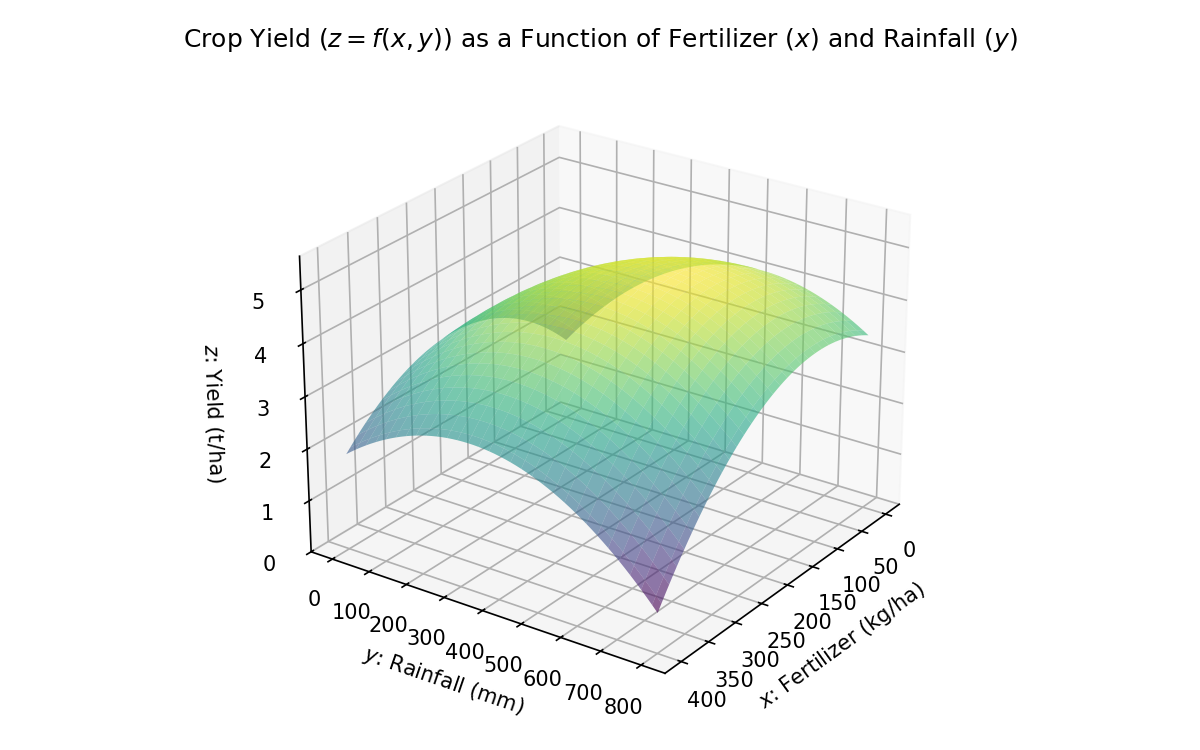
Illustrative surface showing crop yield as a function of fertilizer and rainfall. — Figure 11.1. Graph of the crop yield $z = f (x, y)$ as a function of fertilizer $x$ and rainfall $y$ .

Because $f$ depends on two variables, its graph lives in three dimensions: the horizontal plane represents $x$ (fertilizer) and $y$ (rainfall), while the vertical axis represents $f (x, y)$ (yield). Although 3D graphs are possible, they can be difficult to interpret—especially for decision-making—so we often use level curves and function traces instead.

Level Curves or Contours

Level curves show where the function has the same value, making it easier to identify trade-offs and regions of interest.

Definition: Level Curve of a Function

For a function of two variables $f (x, y)$ , a level curve (or contour) is the set of all points $(x, y)$ in the domain where the function takes a fixed constant value $k$ :

$f (x, y) = k$

In the $x y$ -plane, a level curve connects all points where $f$ produces the same output.

Example: Level Curves for Crop Yield

In the crop yield model, a level curve for $f$ represents all combinations of fertilizer and rainfall that yield the same harvest.

For a fixed yield $z_{0}$ , the level curve is:

${(x, y) ∣ f (x, y) = z_{0}}$

For example, the level curve for $f (x, y) = 4.4 t/ha$ shows all fertilizer-rainfall combinations producing a yield of $4.4$ tonnes per hectare.

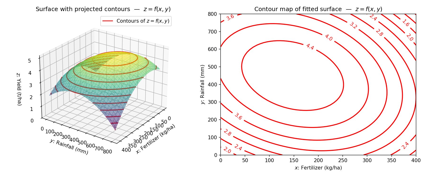
Contour plot showing combinations of fertilizer and rainfall with equal crop yield. — Figure 11.2. Level curves (contours) of crop yield.

From a contour plot, we can answer questions such as:

"If I want $4.4$ t/ha, how can I trade fertilizer for rainfall?"
"Where is the optimal combination of fertilizer and rainfall for maximum yield?"

Level curves are especially useful for visualizing decision boundaries and trade-offs when multiple factors influence an outcome.

Function Traces

Function traces help us examine cross-sections of the surface by fixing one variable and varying the other.

Definition: Trace of a Function

For $f (x, y)$ , a trace is obtained by fixing one variable and letting the other vary:

Trace in the $x$ -direction. Fix $y = c$ and consider

$z = f (x, c)$

This curve lies in the vertical plane parallel to the $x z$ -plane.

Trace in the $y$ -direction. Fix $x = c$ and consider

$z = f (c, y)$

This curve lies in the vertical plane parallel to the $yz$ -plane.

Example: Function Traces for Crop Yield

For the crop yield model, traces show how yield changes when one input is fixed and the other is allowed to vary.

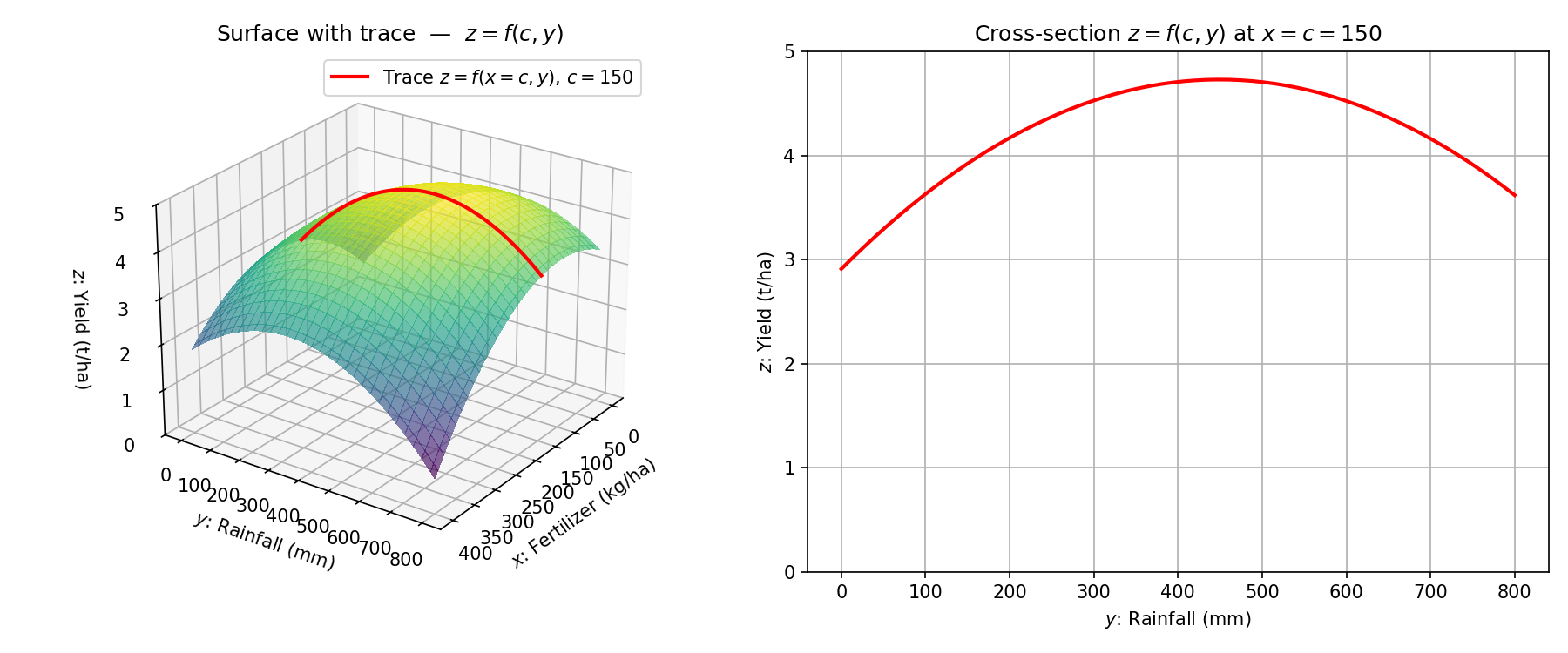
First, fix fertilizer at $150$ kg/ha and vary rainfall. The trace shows how yield changes with rainfall for that fertilizer level.

Trace showing crop yield as rainfall varies while fertilizer is fixed. — Figure 11.3. Trace: Yield vs Rainfall with Fertilizer fixed at $150$ kg/ha.

Second, fix rainfall at $450$ mm and vary fertilizer. The trace shows how yield changes with fertilizer for that rainfall level.

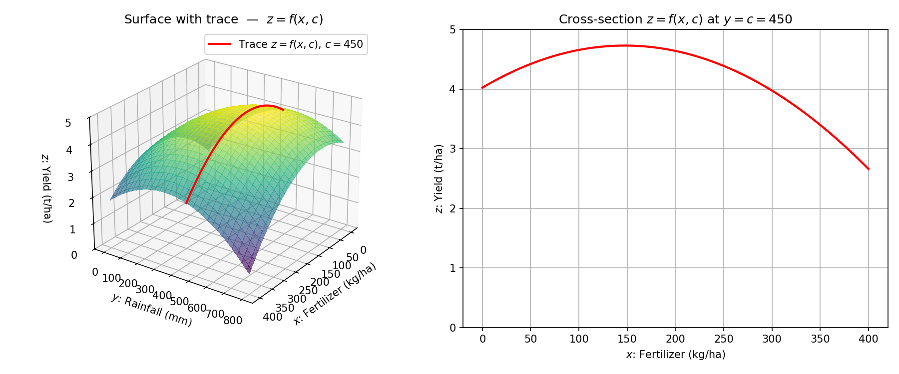
Trace showing crop yield as fertilizer varies while rainfall is fixed. — Figure 11.4. Trace: Yield vs Fertilizer with Rainfall fixed at $450$ mm.

From these traces, we can identify thresholds, such as the fertilizer amount beyond which adding more no longer increases yield.

Interpreting Level Curves and Traces

When a formula is available, finding level curves and traces reduces to substituting a fixed value or solving an equation. The algebraic and graphical techniques are the same as those used for curves in two dimensions, but here they are applied to cross-sections and slices of surfaces. For a conceptual model such as the crop-yield example, the same representations can instead be interpreted directly from a graph or data visualization.

Examples: Domains and Ranges of Multivariable Functions

The following examples show how domain restrictions come from the algebraic form of the function.

Find the domain and range of each function.

Linear function. First, consider

$f (x, y) = 3 x + 5 y + 2,$

There are no algebraic restrictions on $x$ or $y$ , so every ordered pair $(x, y) \in R^{2}$ is allowed. Therefore, the domain is $R^{2}$ .

The expression can produce any real output, so the range is $R$ .
Square-root function. Next, consider

$g (x, y) = 9 - x^{2} - y^{2},$

For the output to be real, the expression under the square root must be non-negative:

$9 - x^{2} - y^{2} \geq 0.$

Therefore, the domain is

${(x, y) \in R^{2} ∣ x^{2} + y^{2} \leq 9} .$

For the range, the square root produces non-negative outputs. Its smallest value is $0$ , and its largest value is $3$ , so the range is $[0, 3]$ .