Chapter 10: Differentiation

Differentiation is the process of finding the derivative of a function, which tells us the slope of the function at a single point on its graph.

In Chapter 4, we defined slope in the context of a linear function. To extend this concept to more general functions, we first define secant lines (slopes over an interval) and then tangent lines (slopes at a single point). These ideas allow us to quantify how a function changes.

Secant & Tangent Lines

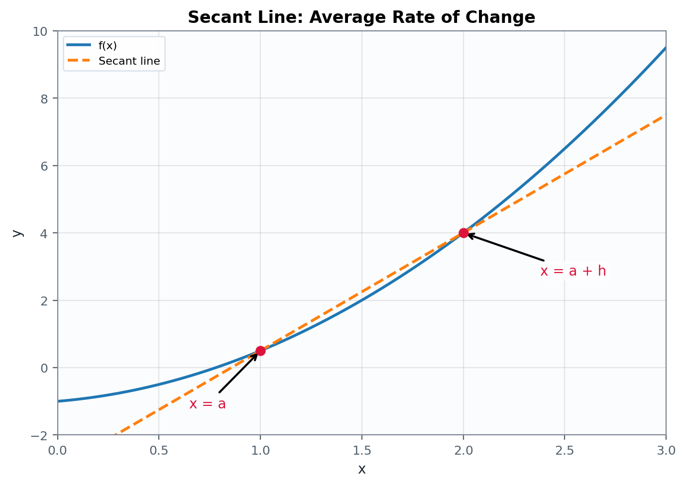
Curve with a secant line through two points on the graph. — Figure 10.1. A secant line approximates the slope of a curve over an interval.

The slope of a secant line to a function at a point $(a, f (a))$ gives an average rate of change of a function between $x = a$ and a nearby point.

To compute it, we pick a value of $x$ close to $a$ , say $x = a + h$ (where $h \neq = 0$ ), and draw a line through the points $(a, f (a))$ , and $(a + h, f (a + h))$ . The slope of this line is:

$m_{sec} = \frac{f ( x ) - f ( a )}{x - a} = \frac{f ( a + h ) - f ( a )}{( a + h ) - a} = \frac{f ( a + h ) - f ( a )}{h}$

Definition: Slope of a Secant Line

Let $f$ be a function defined on an interval $I$ containing $a$ . If $h \neq = 0$ and $a + h \in I$ , the slope of the secant line is:

$m_{sec} = \frac{f ( a + h ) - f ( a )}{h} .$

This expression is also called the difference quotient.

Example: Slope of a Secant Line

This computation turns the geometric idea of a secant line into an average rate of change.

Find the slope of the secant line to the graph of $f (x) = x^{2}$ between $x = 3$ and $x = 5$ .

The two points on the graph are

$(3, f (3)) = (3, 9) and (5, f (5)) = (5, 25) .$

Thus, the secant slope is

$m_{sec} = \frac{f ( 5 ) - f ( 3 )}{5 - 3} = \frac{25 - 9}{2} = 8.$

This value is the average rate of change of $f (x) = x^{2}$ on the interval from $x = 3$ to $x = 5$ .

Definition: Tangent Line

Let $f (x)$ be a function defined in an open interval containing $a$ . The tangent line to $f$ at $x = a$ is the line passing through $(a, f (a))$ with slope:

$m_{tan} = h \to 0 lim \frac{f ( a + h ) - f ( a )}{h}$

provided this limit exists.

Example: Tangent Slope for a Square Root Function

To find a tangent slope, we let the second point move toward the first using the limit definition.

Find the slope of the tangent line to the graph of $f (x) = x$ at $x = 4$ .

$m_{tan} = h \to 0 lim \frac{f ( 4 + h ) - f ( 4 )}{h} = h \to 0 lim \frac{4 + h - 4}{h} = h \to 0 lim (\frac{4 + h + 2}{4 + h + 2}) \cdot \frac{4 + h - 2}{h} = h \to 0 lim \frac{( 4 + h + 2 ) \cdot ( 4 + h - 2 )}{( 4 + h + 2 ) \cdot h} = h \to 0 lim \frac{4 + h ^{2} - 2 ^{2}}{( 4 + h + 2 ) \cdot h} = h \to 0 lim \frac{4 + h - 4}{( 4 + h + 2 ) \cdot h} = h \to 0 lim \frac{h}{( 4 + h + 2 ) \cdot h} = h \to 0 lim \frac{1}{4 + h + 2} = \frac{1}{4 + 2} = \frac{1}{2 + 2} = \frac{1}{4}$

The Derivative of a Function

Definition: The Derivative of a Function

Let $f : (a, b) \to R$ be a function. The derivative of $f$ at $x$ is:

$f^{'} (x) = h \to 0 lim \frac{f ( x + h ) - f ( x )}{h}$

provided the limit exists. If the limit exists for all $x \in (a, b)$ , we say that $f$ is differentiable on $(a, b)$ .

Note that instead of writing $f^{'} (x)$ , we can also write $\frac{df}{d x}$ or $\frac{d}{d x} f (x)$ . All three expressions denote the derivative of $f$ with respect to $x$ .

The prime notation $f^{'} (x)$ is concise and often used in basic calculus or when the variable is clear from context.

The Leibniz notation $\frac{df}{d x}$ , on the other hand, emphasizes the operation of differentiation and explicitly indicates the variable, making it useful in contexts with, e.g., several variables or when applying rules like the chain rule.

Example: The Derivative of a Linear Function

Consider the linear function $f (x) = a x + b, a \neq = 0, b \in R$ . For any $x \in R$ , we compute the derivative of the function as follows:

$f^{'} (x) f^{'} (x) f^{'} (x) f^{'} (x) = h \to 0 lim \frac{( a ( x + h ) + b ) - ( a x + b )}{h} = h \to 0 lim \frac{( a x + ah + b ) - ( a x + b )}{h} = h \to 0 lim \frac{a x + ah + b - a x - b}{h} = h \to 0 lim \frac{ah}{h} = h \to 0 lim a = a$

This makes sense, as a linear function is a straight line with constant slope.

Example: The Derivative of a Quadratic Function

Consider the quadratic function $f (x) = a x^{2}$ , for any $x \in R$ . We compute the derivative of the function, using the limit laws, as follows:

$f^{'} (x) = h \to 0 lim \frac{a ( x + h ) ^{2} - a x ^{2}}{h} = a \cdot h \to 0 lim \frac{( x + h ) ^{2} - x ^{2}}{h} = a \cdot h \to 0 lim \frac{x ^{2} + h ^{2} + 2 h x - x ^{2}}{h} = a \cdot h \to 0 lim \frac{h ^{2} + 2 h x}{h} = a \cdot h \to 0 lim \frac{h ( h + 2 x )}{h} = a \cdot h \to 0 lim (h + 2 x) = 2 a x$

Common Derivatives

Rules: Common Derivatives

Below is a table of some of the most frequently used derivatives. Here $k, n \in R$ , $n \neq = 0$ , $a > 0$ , and the power rule is applied at points where $x^{n}$ is real-valued and differentiable. In particular, the rule holds for every real $n$ when $x > 0$ , and nonzero integer powers can be used on their usual domains. The case $n = 0$ is covered by the constant rule. The trigonometric rules assume that angles are measured in radians.

Table 10.1. Common derivative rules.

Function $f (x)$	Derivative $f^{'} (x)$	Notes
$k$	$0$	Constant rule
$x^{n}$	$n x^{n - 1}$	Power rule, on its differentiable domain
$ln (x)$	$\frac{1}{x}$	$x > 0$
$e^{x}$	$e^{x}$	-
$a^{x}$	$ln (a) a^{x}$	$a > 0$
$sin (x)$	$cos (x)$	-
$cos (x)$	$- sin (x)$	-

Common Differentiation Rules

Rules: Differentiating Combinations of Functions

Just like for limits, there are certain rules that we can apply when differentiating functions. In this context, let $f$ and $g$ be differentiable functions on an interval. For the quotient rule, we additionally require $g (x) \neq = 0$ at the point under consideration. The following rules then hold:

Table 10.2. Rules for differentiating combinations of functions.

Rule	Formula	Name
Sum/Difference	$\frac{d}{d x} (f (x) \pm g (x)) = f^{'} (x) \pm g^{'} (x)$	Sum/Difference Rule
Product	$\frac{d}{d x} (f (x) g (x)) = f^{'} (x) g (x) + f (x) g^{'} (x)$	Product Rule
Quotient	$\frac{d}{d x} (\frac{f ( x )}{g ( x )}) = \frac{f ^{'} ( x ) g ( x ) - f ( x ) g ^{'} ( x )}{( g ( x ) ) ^{2}}$	Quotient Rule
Constant Multiple	$\frac{d}{d x} (k f (x)) = k f^{'} (x), k \in R$	Constant Multiple Rule

Example: Applying the Product Rule

Here is how the derivative table combines with the product rule in a concrete calculation.

Using the rules in the table, compute the derivative of the function $h (x) = e^{x} sin (x)$ .

Letting $f (x) = e^{x}$ and $g (x) = sin (x)$ , we get $f^{'} (x) = e^{x}$ and $g^{'} (x) = cos (x)$ . Following the order $f^{'} g + f g^{'}$ in the product rule gives

$h^{'} (x) = e^{x} sin (x) + e^{x} cos (x) = e^{x} (sin (x) + cos (x)) .$

Expanding the final expression returns the previous line, which checks the factorization.

Example: Product and Quotient Rules

This example applies the product and quotient rules to the same pair of functions so that the two calculations can be compared directly.

Let

$f (x) = 2 x^{2} and g (x) = x .$

Their derivatives are

$f^{'} (x) = 4 x and g^{'} (x) = 1.$

First, apply the product rule while keeping $f$ and $g$ separate:

$(f (x) g (x))^{'} = \frac{d}{d x} (f (x) g (x)) = f^{'} (x) g (x) + f (x) g^{'} (x) = 4 x \cdot x + 2 x^{2} \cdot 1 = 6 x^{2}$

Next, apply the quotient rule. Since $g (x) = x$ , the quotient is defined only when $x \neq = 0$ :

$(\frac{f ( x )}{g ( x )})^{'} = \frac{d}{d x} (\frac{f ( x )}{g ( x )}) = \frac{4 x \cdot x - 2 x ^{2} \cdot 1}{x ^{2}} = \frac{2 x ^{2}}{x ^{2}} = 2$

Thus, the derivative of the quotient is $2$ at every point $x \neq = 0$ in its domain. The simplification does not define the original quotient or its derivative at $x = 0$ .

The Chain Rule

We have seen the techniques for differentiating basic functions as well as sums, differences, products, quotients, and constant multiples of these functions. However, these techniques do not allow us to differentiate compositions of functions. In this section, we study the rule for finding the derivative of the composition of two or more functions.

Rule: The Chain Rule

Function composition diagram showing the mappings from the domain through an intermediate set to the codomain. — Figure 10.2. Function composition: the output of $g$ becomes the input of $f$ .

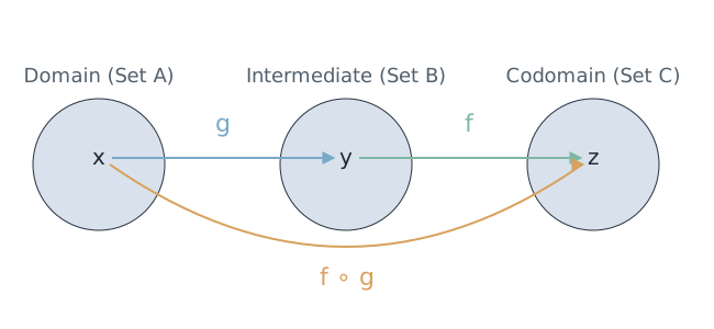
Let $f$ and $g$ be functions such that:

$g$ is differentiable at $x$
$f$ is differentiable at $g (x)$

For the composite function:

$h (x) = (f \circ g) (x) = f (g (x))$

the derivative is then defined as:

$\frac{d}{d x} (f \circ g) (x) = f^{'} (g (x)) \cdot g^{'} (x)$

Method: Applying the Chain Rule

To differentiate $h (x) = f (g (x))$ , follow the steps:

Identify the outer function $f (x)$ and the inner function $g (x)$
Differentiate $f$ with respect to its argument to get $f^{'} (x)$
Evaluate $f^{'} (g (x))$ by substituting $g (x)$ into $f^{'} (x)$
Differentiate $g$ with respect to its argument to get $g^{'} (x)$
Compute $h^{'} (x)$ as $f^{'} (g (x)) \cdot g^{'} (x)$

Example: Differentiating a Square of Sine

For this composition, identify the outer square and the inner sine function before applying the chain rule.

Differentiate $h (x) = (sin (x))^{2}$ .

To do so, we let:

The outer function be $f (u) = u^{2}$ , so $f^{'} (u) = 2 u$
The inner function be $g (x) = sin (x)$ , so $g^{'} (x) = cos (x)$

Applying the Chain Rule, we then get:

$h^{'} (x) = f^{'} (g (x)) \cdot g^{'} (x) = 2 sin (x) \cdot cos (x)$

Example: Differentiating an Exponential Composite Function

Here the exponent contains a polynomial, so the exponential function is the outer function.

Differentiate $f (x) = e^{x^{3} + 1}$ .

To do so, we let:

The outer function be $f (u) = e^{u}$ , so $f^{'} (u) = e^{u}$ .
The inner function be $g (x) = x^{3} + 1$ , so $g^{'} (x) = 3 x^{2}$ .

Applying the Chain Rule, we then get:

$f^{'} (x) = e^{x^{3} + 1} \cdot 3 x^{2} = 3 x^{2} e^{x^{3} + 1} .$

Finding Extrema

In this section, we focus on an important application of derivatives: finding maxima and minima of functions.

Definitions: Local Minima and Maxima

These terms describe extreme values near a point.

Let $f$ be defined on a domain containing $c$ .

Local minimum. The value $f (c)$ is a local minimum if there is an open interval around $c$ such that $f (c) \leq f (x)$ for all points $x$ in that interval that also belong to the domain.

Local maximum. The value $f (c)$ is a local maximum if there is an open interval around $c$ such that $f (c) \geq f (x)$ for all points $x$ in that interval that also belong to the domain.

By contrast, $f (c)$ is an absolute minimum or absolute maximum on an interval $I$ if the corresponding inequality holds for every $x \in I$ . Local and absolute maxima and minima are collectively called extrema.

Theorem: The Extreme Value Theorem

Let $f$ be a continuous function defined on a closed, bounded interval $[a, b]$ . Then $f$ has both an absolute maximum and an absolute minimum value on $[a, b]$ .

The Turning Point of a Quadratic Function

Recall from Chapter 4 that a turning point of a graph is a point at which the graph changes direction from increasing to decreasing or vice versa. For a quadratic function, this point is also called the vertex. If $f (x) = a x^{2} + b x + c$ with $a \neq = 0$ , the turning point is:

$T = (- \frac{b}{2 a}, - \frac{Δ}{4 a}), with Δ = b^{2} - 4 a c$

We will later see how to derive this point by setting the first derivative of the function to zero and solving for $x$ (i.e., $f^{'} (x) = 0$ ).

For $h (x) = 6 x^{2} + 11 x + 3$ , with discriminant $Δ = 49$ , the turning point is:

$x_{T} y_{T} = - \frac{b}{2 a} = - \frac{11}{2 \cdot 6} = - \frac{11}{12} \approx - 0.917 = - \frac{Δ}{4 a} = - \frac{49}{4 \cdot 6} = - \frac{49}{24} \approx - 2.042$

Since $a = 6 > 0$ , the parabola opens upwards, and the turning point is the minimum point. This can also be confirmed by inspecting the graph.

Derivatives & Local Extrema

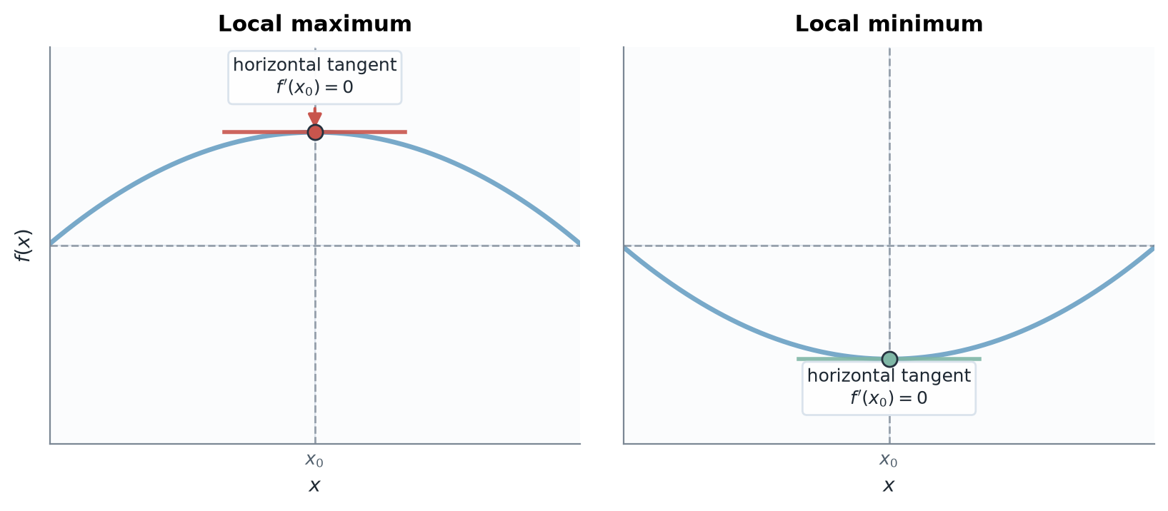
The derivative $f^{'} (x)$ measures the slope of the tangent line at $(x, f (x))$ . If $f$ is differentiable at an interior input $c$ and has a local maximum or minimum there, then

$f^{'} (c) = 0.$

This result is sometimes called Fermat's theorem. An interior number $c$ in the domain is called a critical number if $f^{'} (c) = 0$ or $f^{'} (c)$ does not exist. If $f (c)$ exists, the corresponding graph point $(c, f (c))$ is called a critical point. Critical numbers are candidates for extrema, but they need not actually produce extrema. Endpoints must also be considered when finding absolute extrema on a closed interval.

Two generic smooth curves showing a local maximum and local minimum, each with a horizontal tangent at x zero. — Figure 10.3. At smooth local extrema, the tangent line is horizontal, so the derivative is zero.

To classify critical numbers, we can use the so-called first derivative sign test or second derivative test.

Test: The First Derivative Sign Test

Let $c$ be an interior number in the domain. Assume that $f$ is continuous at $c$ and differentiable on intervals immediately to the left and right of $c$ .

If $f^{'}$ changes from positive to negative at $c$ , then $f$ has a local maximum there.
If $f^{'}$ changes from negative to positive at $c$ , then $f$ has a local minimum there.
If $f^{'}$ is positive on both sides of $c$ , or negative on both sides, then $f$ has no local extremum there.

If $f^{'}$ is zero throughout part of a neighboring interval, this simple sign test may be inconclusive. The behavior on the flat interval should then be checked directly from the definition of a local extremum.

Test: The Second Derivative Test

Suppose that $f^{'} (c) = 0$ . If $f^{''} (c)$ exists, then

If $f^{''} (c) > 0$ we have a local minimum
If $f^{''} (c) < 0$ we have a local maximum
If $f^{''} (c) = 0$ , the test gives no information

If $f^{''} (c)$ does not exist, the test does not apply.

Method: Finding Local Extrema

To find local extrema using derivatives:

Compute the first derivative $f^{'} (x)$ .
Find the critical numbers in the domain, where $f^{'} (x) = 0$ or where $f^{'} (x)$ is undefined.
Use the first derivative sign test or, when applicable, the second derivative test to classify each critical number.
Substitute each classified critical number into $f (x)$ to find the corresponding function value.

If $f$ is continuous on a closed interval $[a, b]$ , it has absolute extrema on that interval. Find all critical numbers in $(a, b)$ , evaluate $f$ at those numbers and at the endpoints, and then compare the values. The largest is the absolute maximum and the smallest is the absolute minimum. If $f$ is not continuous on $[a, b]$ , this candidate comparison is not sufficient without further analysis.

Warning: Critical Numbers Are Candidates

The equation $f^{'} (x) = 0$ identifies candidates, not guaranteed extrema. A derivative may equal zero without changing from increasing to decreasing or vice versa. Likewise, an extremum can occur at an endpoint or at an input where the derivative does not exist.

Example: Finding Local Maxima and Minima

The derivative tests turn this optimization question into finding and classifying critical numbers.

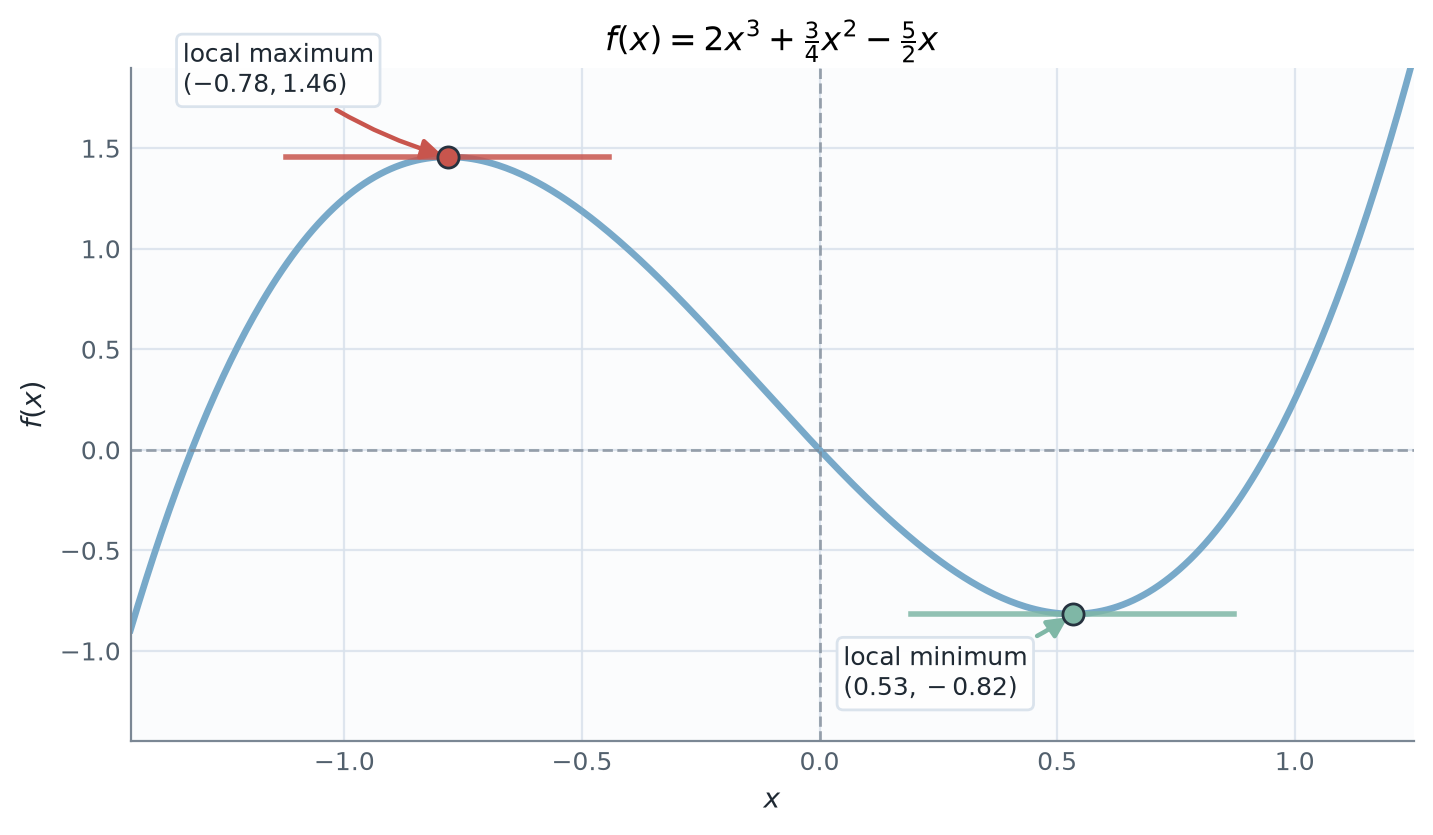
Find the local maxima and minima of the function $f (x) = 2 x^{3} + \frac{3}{4} x^{2} - \frac{5}{2} x$ .

We differentiate $f$ and obtain

$f^{'} (x) = 6 x^{2} + 2 \cdot \frac{3}{4} x - \frac{5}{2} = 6 x^{2} + \frac{3}{2} x - \frac{5}{2}$

In order to find the critical numbers where $f^{'} (x) = 0$ , we solve the quadratic equation $6 x^{2} + \frac{3}{2} x - \frac{5}{2} = 0$ . The discriminant is $Δ = (\frac{3}{2})^{2} - 4 \cdot 6 \cdot (- \frac{5}{2}) = \frac{249}{4}$ and the roots are thus

$x_{1} x_{2} = \frac{- \frac{3}{2} - \frac{249}{4}}{2 \cdot 6} \approx - 0.78, = \frac{- \frac{3}{2} + \frac{249}{4}}{2 \cdot 6} \approx 0.53$

Differentiating once again, we obtain

$f^{''} (x) = 12 x + \frac{3}{2}$

and by calculation, $f^{''} (x_{1}) < 0$ and $f^{''} (x_{2}) > 0$ . Thus, $f$ has a local maximum at $x_{1}$ and a local minimum at $x_{2}$ . The corresponding critical points are $(x_{1}, f (x_{1})) = (- 0.78, 1.46)$ and $(x_{2}, f (x_{2})) = (0.53, - 0.82)$ .

A plot of the cubic function with its local maximum and local minimum marked. — Figure 10.4. The critical numbers found from $f^{'} (x) = 0$ correspond to a local maximum point and a local minimum point on the graph.

Keyboard shortcuts

Mathematics Brush-up for Data Science