Chapter 7: Differentiation

Differentiation

Differentiation is the process of finding the derivative of a function, which tells us the slope of the function at a single point on its graph.

In an earlier chapter, we defined the slope in the context of a linear function. To extend this concept to more general functions, we first define secant lines (slopes over an interval) and then tangent lines (slopes at a single point). These ideas allow us to quantify how a function changes.

Secant & Tangent Lines

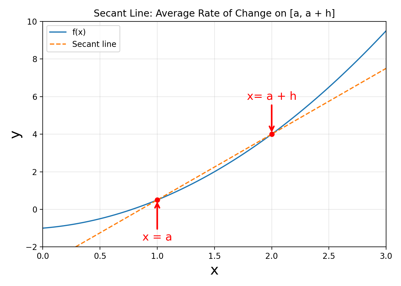
The slope of a secant line to a function at a point $(a, f (a))$ gives an average rate of change of a function between $x = a$ and a nearby point.

To compute it, we pick a value of $x$ close to $a$ , say $x = a + h$ (where $h \neq = 0$ ), and draw a line through the points $(a, f (a))$ , and $(a + h, f (a + h))$ . The slope of this line is:

$m_{sec} = \frac{f ( x ) - f ( a )}{x - a} = \frac{f ( a + h ) - f ( a )}{( a + h ) - a} = \frac{f ( a + h ) - f ( a )}{h}$

Definition: Slope of a Secant Line

Let $f$ be a function defined on an interval $I$ containing $a$ . If $h \neq = 0$ and $a + h \in I$ , the slope of the secant line is:

$m_{sec} = \frac{f ( a + h ) - f ( a )}{h} .$

This expression is also called the difference quotient.

Example: Slope of a Secant Line

Find the slope of the tangent line to the graph of $f (x) = x^{2}$ at $x = 3$ .

$m_{t an} = h \to 0 lim \frac{f ( 3 + h ) - f ( 3 )}{h} = h \to 0 lim \frac{( 3 + h ) ^{2} - 9}{h} = h \to 0 lim \frac{9 + 6 h + h ^{2} - 9}{h} = h \to 0 lim \frac{h ( 6 + h )}{h} = h \to 0 lim 6 + h = 6$

Definition: Tangent Line

Let $f (x)$ be a function defined in an open interval containing $a$ . The tangent line to $f$ at $x = a$ is the line passing through $(a, f (a))$ with slope:

$m_{tan} = h \to 0 lim \frac{f ( a + h ) - f ( a )}{h}$

provided this limit exists.

Example: Tangent Line

Find the slope of the tangent line to the graph of $f (x) = x$ at $x = 4$ .

$m_{tan} = h \to 0 lim \frac{f ( 4 + h ) - f ( 4 )}{h} = h \to 0 lim \frac{4 + h - 4}{h} = h \to 0 lim (\frac{4 + h + 2}{4 + h + 2}) \cdot \frac{4 + h - 2}{h} = h \to 0 lim \frac{( 4 + h + 2 ) \cdot ( 4 + h - 2 )}{( 4 + h + 2 ) \cdot h} = h \to 0 lim \frac{4 + h ^{2} - 2 ^{2}}{( 4 + h + 2 ) \cdot h} = h \to 0 lim \frac{4 + h - 4}{( 4 + h + 2 ) \cdot h} = h \to 0 lim \frac{h}{( 4 + h + 2 ) \cdot h} = h \to 0 lim \frac{1}{4 + h + 2} = \frac{1}{4 + 2} = \frac{1}{2 + 2} = \frac{1}{4}$

The Derivative of a Function

Definition: The Derivative of a Function

Let $f : (a, b) \to R$ be a function. The derivative of $f$ at $x$ is:

$f^{'} (x) = h \to 0 lim \frac{f ( x + h ) - f ( x )}{h}$

provided the limit exists. If the limit exists for all $x \in (a, b)$ , we say that $f$ is differentiable on $(a, b)$ .

Note that instead of writing $f^{'} (x)$ , we can also write $\frac{df}{d x}$ or $\frac{d}{d x} f (x)$ . All three expressions denote the derivative of $f$ with respect to $x$ .

The prime notation $f^{'} (x)$ is concise and often used in basic calculus or when the variable is clear from context.

The Leibniz notation $\frac{df}{d x}$ , on the other hand, emphasizes the operation of differentiation and explicitly indicates the variable, making it useful in contexts with, e.g., several variables or when applying rules like the chain rule.

Note that instead of writing $f^{'} (x)$ we sometimes write $\frac{df}{d x}$ or $\frac{d}{d x} f (x)$ , i.e., these expressions are equivalent, but ...

Example: The Derivative of a Linear Function

Consider the linear function $f (x) = a x + b, a \neq = 0, b \in R$ . For any $x \in R$ . We compute the derivative of the function, as follows:

$f^{'} (x) f^{'} (x) f^{'} (x) f^{'} (x) = h \to 0 lim \frac{( a ( x + h ) + b ) - ( a x + b )}{h} = h \to 0 lim \frac{( a x + ah + b ) - ( a x + b )}{h} = h \to 0 lim \frac{a x + ah + b - a x - b}{h} = h \to 0 lim \frac{ah}{h} = h \to 0 lim a = a$

This makes sense, as a linear function is a straight line with constant slope.

Example: The Derivative of a Quadratic Function

Consider the quadratic function $f (x) = a x^{2}$ , for any $x \in R$ . We compute the derivative of the function, using the limit laws, as follows:

$f^{'} (x) = h \to 0 lim \frac{a ( x + h ) ^{2} - a x ^{2}}{h} = a \cdot n \to \infty lim \frac{( x + h ) ^{2} - x ^{2}}{h} = a \cdot h \to 0 lim \frac{x ^{2} + h ^{2} + 2 h x - x ^{2}}{h} = a \cdot h \to 0 lim \frac{h ^{2} + 2 h x}{h} = a \cdot h \to 0 lim \frac{h ( h + 2 x )}{h} = a \cdot h \to 0 lim h + 2 x = 2 a x$

Common Derivatives

Below is a table of some of the most frequently used derivatives. Here $k, a \in R$ , $a > 0$ , and $n \neq = 0$ .

Function $f (x)$	Derivative $f^{'} (x)$	Notes
$k$	$0$	Constant rule
$x^{n}$	$n x^{n - 1}$	Power rule
$ln (x)$	$\frac{1}{x}$	$x > 0$
$e^{x}$	$e^{x}$	-
$a^{x}$	$ln (a) a^{x}$	$a > 0$
$sin (x)$	$cos (x)$	-
$cos (x)$	$- sin (x)$	-

Example: ...

Using the rules in the table, compute the derivative of the function $h (x) = e^{x} sin (x)$ .

Letting $f (x) = e^{x}$ and $g (x) = sin (x)$ , we get from the table of derivatives that $f^{'} (x) = e^{x}$ and $g^{'} (x) = cos (x)$ . The product rule then gives

$h^{'} (x) = \frac{d}{d x} (e^{x} sin (x)) = e^{x} sin (x) + e^{x} cos (x) = e^{x} (sin (x) + cos (x))$

Common Differentiation Rules

Just like for limits, there are certain rules that we can apply when differentiating functions. In this context, let $f$ and $g$ be differentiable functions on an interval, with $g (x) \neq = 0$ . The following rules then hold:

Rule	Formula	Name
Sum/Difference	$\frac{d}{d x} (f (x) \pm g (x)) = f^{'} (x) \pm g^{'} (x)$	Sum/Difference Rule
Product	$\frac{d}{d x} (f (x) g (x)) = f^{'} (x) g (x) + f (x) g^{'} (x)$	Product Rule
Quotient	$\frac{d}{d x} (\frac{f ( x )}{g ( x )}) = \frac{f ^{'} ( x ) g ( x ) - f ( x ) g ^{'} ( x )}{( g ( x ) ) ^{2}}$	Quotient Rule
Constant Multiple	$\frac{d}{d x} (k f (x)) = k f^{'} (x), k \in R$	Constant Multiple Rule

Example:

Differentiate the functions $f (x) = 2 x^{2}$ , $g (x) = x$ , and consider the derivative of the product $f (x) \cdot g (x)$ and the quotient $\frac{f ( x )}{g ( x )}$ , without performing algebraic manipulations until the very end.

We already know that

$f^{'} (x) = \frac{d}{d x} (2 x^{2}) = 2 \cdot 2 \cdot x = 4 x and g^{'} (x) = \frac{d}{d x} (x) = 1$

Now, computing the product, we get:

$(f (x) g (x))^{'} = \frac{d}{d x} (f (x) g (x)) = f^{'} (x) g (x) + f (x) g^{'} (x) = 4 x \cdot x + 2 x^{2} \cdot 1 = 6 x^{2}$

For the quotient, where we assume $x \neq = 0$ , as $g (x)$ otherwise would be zero, we get:

$(\frac{f ( x )}{g ( x )})^{'} = \frac{d}{d x} \frac{f ( x )}{g ( x )} = \frac{4 x \cdot x - 2 x ^{2} \cdot 1}{x ^{2}} = \frac{2 x ^{2}}{x ^{2}} = 2$

The Chain Rule

We have seen the techniques for differentiating basic functions as well as sums, differences, products, quotients, and constant multiples of these functions. However, these techniques do not allow us to differentiate compositions of functions. In this section, we study the rule for finding the derivative of the composition of two or more functions.

Definition: The Chain Rule

Let $f$ and $g$ be functions such that:

$g$ is differentiable at $x$
$f$ is differentiable at $g (x)$

For the composite function:

$h (x) = (f \circ g) (x) = f (g (x))$

the derivative is then defined as:

$\frac{d}{d x} (f \circ g) (x) = f^{'} (g (x)) \cdot g^{'} (x)$

Recipie: Applying the Chain Rule

To differentiate $h (x) = f (g (x))$ , follow the steps:

Identify the outer function $f (x)$ and the inner function $g (x)$
Differentiate $f$ with respect to its argument to get $f^{'} (x)$
Evaluate $f^{'} (g (x))$ by substituting $g (x)$ into $f^{'} (x)$
Differentiate $g$ with respect to its argument to get $g^{'} (x)$
Compute $h^{'} (x)$ as $f^{'} (g (x)) \cdot g^{'} (x)$

Definition:

Differentiate $h (x) = (sin (x))^{2}$ .

To do so, we let:

The outer function be $f (u) = u^{2}$ , so $f^{'} (u) = 2 u$
The inner function be $g (x) = sin (x)$ , so $g^{'} (x) = cos (x)$

Applying the Chain Rule, we then get:

$h^{'} (x) = f^{'} (g (x)) \cdot g^{'} (x) = 2 sin (x) \cdot cos (x)$

Example:

Differentiate $f (x) = e^{x^{3} + 1}$ .

To do so, we let:

The outer function be $f (u) = e^{u}$ , so $f^{'} (u) = e^{u}$ .
The inner function be $g (x) = x^{3} + 1$ , so $g^{'} (x) = 3 x^{2}$ .

Applying the Chain Rule, we then get:

$f^{'} (x) = e^{x^{3} + 1} \cdot 3 x^{2} = 3 x^{2} e^{x^{3} + 1} .$

Finding Extrema

In this section, we focus on an important application of derivatives: finding maxima and minima of functions.

Definition: Local Minima and Maxima

Let $f$ be defined on an interval $I$ containing $x$ , then:

$f (c)$ is the minimum of $f$ on $I$ if $f (c) \leq f (x)$ for all $x \in I$
$f (c)$ is the maximum of $f$ on $I$ if $f (c) \geq f (x)$ for all $x \in I$

The maximum and minimum values are the extreme values, or extrema, of $f$ on $I$ .

Definition: The Extreme Value Theorem

Let $f$ be a continuous function defined on a closed interval $I$ . Then $f$ has both a maximum and minimum value on $I$ .

The Turning Point of a Quadratic Function

Recall from earlier, a turning point (or tipping point) of a graph is a point at which the graph changes direction from increasing to decreasing or vice versa. For a quadratic formula, the formula for the turning point is:

$T = (- \frac{b}{2 a}, - \frac{Δ}{4 a}), with Δ = b^{2} - 4 a c$

We will later see how to find derive this point by setting the first derivative of the function to zero and solving for $x$ (i.e., $f^{'} (x) = 0$ ).

For $h (x) = 6 x^{2} + 11 x + 3$ , with discriminant $D = 49$ , the turning point is:

$x_{T} y_{T} = - \frac{b}{2 a} = - \frac{11}{2 \cdot 6} = - \frac{11}{12} \approx - 0.917 = - \frac{D}{4 a} = - \frac{49}{4 \cdot 6} = - \frac{49}{24} \approx - 2.042$

Since $a = 6 > 0$ , the parabola opens upwards, and the turning point is a minimum. This can also be confirmed by inspecting the graph.

Derivatives & Local Extrema

The derivative $f^{'} (x)$ measures the slope of the tangent line at $(x, f (x))$ . At a local maximum or minimum, the tangent line is horizontal, meaning:

$f^{'} (x_{0}) = 0 or f^{'} (x_{0}) is undefined$

Such points are also called critical points.

Definition: The Second Derivative Test

Let $f$ be a 2-times differentiable function and $x_{0}$ a point such that $f^{'} (x_{0}) = 0$ . Then

If $f^{''} (x_{0}) > 0$ we have a local minimum
If $f^{''} (x_{0}) < 0$ we have a local maximum
If $f^{''} (x_{0}) = 0$ or doesn't exist, the test gives no information

Example: Finding Local Maxima and Minima

Find the local maxima and minima of the function $f (x) = 2 x^{3} + \frac{3}{4} x^{2} - \frac{5}{2} x$ .

We differentiate $f$ and obtain

$f^{'} (x) = 6 x^{2} + 2 \cdot \frac{3}{4} x - \frac{5}{2} = 6 x^{2} + \frac{3}{2} x - \frac{5}{2}$

In order to find the points where $f^{'} (x) = 0$ we solve the quadratic equation $6 x^{2} + \frac{3}{2} x - \frac{5}{2} = 0$ . The discriminant is $D = (\frac{3}{2})^{2} - 4 \cdot 6 \cdot (- \frac{5}{2}) = \frac{249}{4}$ and the roots are thus

$x_{1} x_{2} = \frac{- \frac{3}{2} - \frac{249}{4}}{2 \cdot 6} \approx 0.53, = \frac{- \frac{3}{2} + \frac{249}{4}}{2 \cdot 6} \approx - 0.78$

Differentiating once again, we obtain

$f^{''} (x) = 12 x + \frac{3}{2}$

and by calculation, $f^{''} (x_{1}) > 0$ and $f^{''} (x_{2}) < 0$ . We can compute the coordinates $(x_{1}, f (x_{1})) = (0.53, - 0.81)$ , $(x_{2}, f (x_{2})) = (- 0.78, 1.45)$

Mathematics Brush-up for Data Science