Chapter 7: Equation Solving
Equations express the equality of two expressions and are essential tools for modeling and solving real-world problems. While a function describes the relationship between variables, solving an equation means finding the variable values that make the equality true. This chapter focuses on linear and quadratic equations, showing how algebraic solutions can also be interpreted geometrically as intersections and roots. Finally, it shows how the sign of a polynomial changes around its roots and uses this idea to solve inequalities.
Chapter 4 introduced two important types of points on the graph of a function: - and -intercepts.
To find the -intercepts, the output is fixed at zero. We solve
for the unknown input . Each solution gives an -intercept .
To find the -intercept, the input is fixed at . Provided that belongs to the domain, we evaluate
The -intercept is therefore the point . This is normally a function-evaluation problem: the input is known, and we calculate the corresponding output.
Thus, fixing an input leads to function evaluation, whereas fixing an output leads to equation solving.
The -intercept problem is a special case of a more general question. Instead of fixing the output at zero, suppose we specify an arbitrary output . We then find the corresponding inputs by solving
for . Graphically, the solutions are the -coordinates of the points where the graph of intersects the horizontal line . When , these points are the -intercepts.
Solving an equation means finding every value of the chosen variable that makes the equality true. Algebraically, we often rearrange the equation, when possible, to isolate that variable on one side and leave quantities that do not involve it on the other.
To solve an equation reliably:
- Record the domain and any restrictions, such as denominators that cannot equal zero or logarithm arguments that must be positive.
- Simplify both sides and use reversible algebraic transformations whenever possible.
- Isolate the chosen variable when possible.
- If a step is not reversible, treat the resulting values as candidates rather than confirmed solutions.
- Check all candidates in the original equation.
- State the final solution set.
An algebraic step is equivalent when it preserves exactly the same solution set. Equivalent steps are reversible: they can be undone. Adding or subtracting the same expression on both sides is reversible, as is multiplying or dividing both sides by the same known nonzero number. In this book, connects equivalent equations.
If a step cannot always be reversed, we use instead. This means that every solution of the equation before the arrow satisfies the equation after it, but the new equation may have additional solutions. Values obtained after such a step are therefore candidates that must be checked in the original equation.
Consider the equation
Subtracting from both sides and then dividing both sides by gives
Both steps can be reversed, so all three equations have the same solution.
Squaring both sides is a common step that cannot always be reversed. If , then
However, for real numbers and ,
The squared equation therefore includes the original case , but it also allows the additional case . Squaring can consequently add solutions that were not present in the original equation. Such values are called extraneous solutions.
For this reason, connect a squaring step with , treat the resulting values as candidates, and check them in the original equation.
Solve
The square root is defined when , so the domain is . Squaring both sides gives a necessary condition:
The candidates are therefore and . Both belong to the domain, but they must still be checked in the original equation:
Thus, the solution set is . The candidate satisfies the squared equation but not the original equation, so it is extraneous.
Solutions to Equations as Roots
The preceding section focused on solving equations through valid algebraic transformations and, when possible, isolating the chosen variable. Another useful formulation places all terms on one side and zero on the other. For an equation between two functions,
Define the difference function
The original equation is then equivalent to . This places the equation in a form that can be interpreted through roots.
A root of a function , also called a zero, is an input value such that .
If is real, the corresponding -intercept is the point on the graph. Thus, a root is a number, while an -intercept is a point.
Consequently, solving is equivalent to finding the real roots of their difference , or graphically the -coordinates of the points where the graph of meets the -axis.
Solving Linear Equations
In this section, we illustrate the equation-solving process for the case where the resulting function is linear. In such cases, solving is equivalent to finding the root of the linear function .
The figure below shows the same equation in two ways: as an intersection problem and as a root-finding problem.
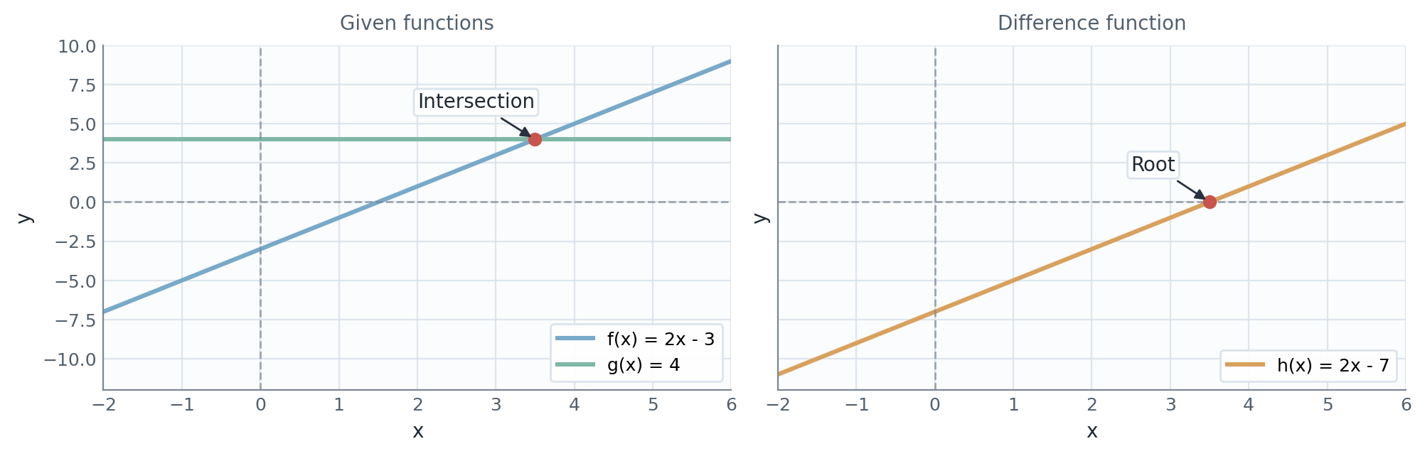
Consider the functions:
Here, is linear and is a constant function.
Finding the intersection of the graphs means determining such that:
We can convert this into a root-finding problem by moving all terms to one side, expressing the equation in the standard form :
Here, the left-hand side can be regarded as a new function . Finding its root is equivalent to solving the original equation:
The solution is the input-coordinate of the point where the graphs of and intersect. In terms of the root-finding approach, it is the root of , and is the corresponding point where the graph of meets the -axis.
Solving Quadratic Equations
In this section, we illustrate the equation-solving process for the case where the resulting difference is quadratic. In such cases, solving is equivalent to finding the root of the quadratic function .
Here the same root-finding idea applies to two quadratic functions, producing two intersection points.
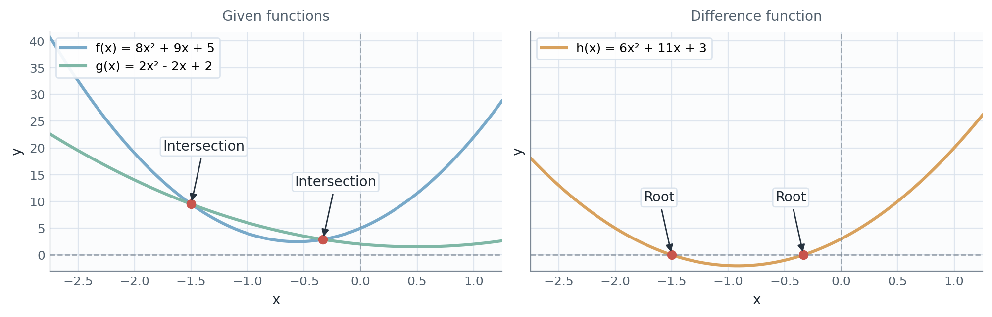
Consider the functions:
Here, and are both quadratic.
Finding the intersection of the graphs means determining such that:
We convert this to a root-finding problem by moving everything to one side:
At this stage, we have reduced the problem to solving a quadratic equation:
There are two standard ways to find its roots:
- By factoring the quadratic expression into a product of two linear factors.
- By applying the quadratic formula, which works even when factoring is not straightforward.
In the examples that follow, we will illustrate both approaches, using the same function .
Solving Via Factorization
Factoring a quadratic expression means expressing it as a product of two linear factors. If this is possible, the zero product property can be applied:
This allows us to solve a quadratic equation by setting each factor equal to zero.
To solve a polynomial equation by factorization:
- Rewrite the equation so one side is .
- Factor the polynomial as a product of simpler factors.
- Use the zero product property by setting each factor equal to .
- Solve the resulting simpler equations.
- Check that the solutions satisfy the original equation.
- State the final solution set.
We are given the quadratic polynomial
and want to factor it using the grouping method introduced in Chapter 6.
The expression contains three terms, but the grouping method requires four. Thus, the first step is to rewrite the trinomial as a four-term polynomial. This can be done using Method: Factoring Trinomials.
Step 1: Identify coefficients:
- is the coefficient of the highest-order term
- is the coefficient of the second-highest-order term
- is the constant term
Step 2: Find two integers , such that
Choosing and satisfies these conditions since and .
Step 3: Rewrite the middle term using and :
Now we can apply the grouping method as described in Method: Factorization by Grouping.
Step 1: Group the terms into pairs:
Step 2: Factor out the greatest common factor (GCF) from each group:
Step 3: A Common binomial factor appears:
Finally, we can now apply the zero product property to solve for :
Solving Via The Quadratic Formula
Another way to find the roots of is to apply the quadratic formula.
Consider the quadratic equation:
where . The solutions of this equation are given by the quadratic formula:
The discriminant determines the number of real solutions:
- If : two distinct real solutions.
- If : one real (repeated) solution.
- If : no real solutions.
The square root denotes the non-negative principal square root. The symbol then tells us to use both its positive and negative signs in the numerator.
To solve the quadratic equation
we set , , and in the formula:
Hence, we get:
These match the solutions obtained by factoring.
Factorized Form and Roots of a Polynomial
Just as quadratic equations can be expressed in factorized form as
higher-order polynomials can sometimes be written as products of real linear factors. This happens when all their roots are real; otherwise, irreducible quadratic factors remain when working over the real numbers.
If a real polynomial of degree has real roots , counted with repetition, then it can be expressed as
where is the leading coefficient and each satisfies . A repeated value in the list represents a root with multiplicity greater than one.
Not every real polynomial has this form using real linear factors. For example, has no real roots and cannot be factored into real linear factors. More generally, a real polynomial factors into real linear factors and irreducible quadratic factors. Over the complex numbers, every degree- polynomial factors into linear factors when multiplicities are counted.
This form reveals several geometric features of the polynomial:
- The number of linear factors equals the degree when all roots are real and multiplicities are counted
- Each distinct real root corresponds to the -intercept
- The coefficient determines the vertical stretch and orientation of the curve. For example, changing its sign reflects the graph across the -axis.
The following examples illustrate how these properties appear graphically.
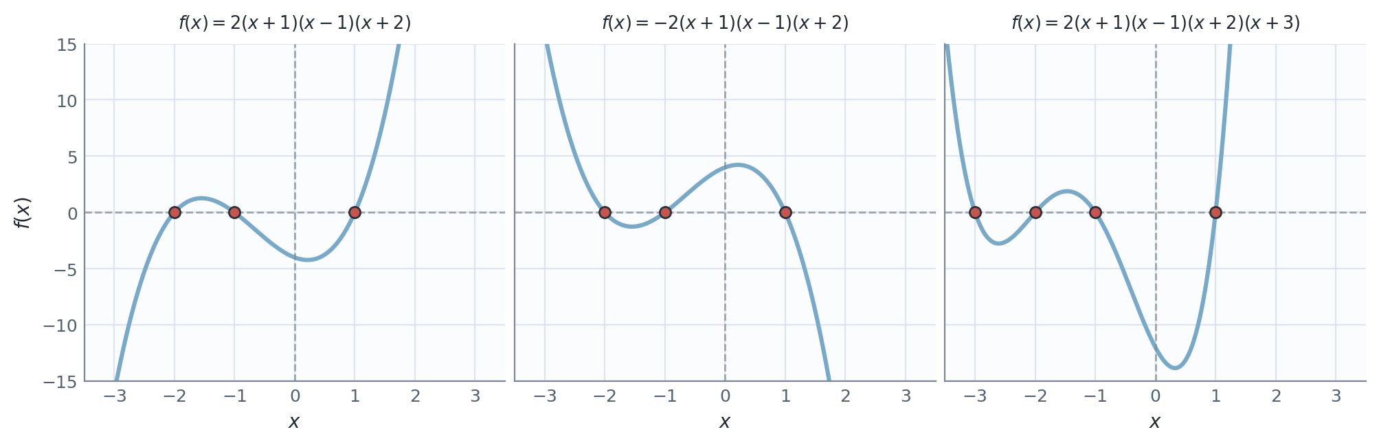
Consider the first polynomial in the plot:
This function has three linear factors, so the polynomial is of degree three. The roots, listed in the order they appear in the algebraic expression, are , , and . At each of these values, one factor becomes zero, defining an -intercept where the graph meets the -axis.
Now look at the second polynomial in the plot:
The only difference is the sign of the leading coefficient. Changing it from to reflects the entire graph across the -axis, while the roots remain in the same order and at the same positions.
Finally, consider the third polynomial in the plot:
Here we have four linear factors, so the polynomial is of degree four. The roots, again listed in the order of the factors, are , , , and . As before, each root defines an -intercept where the graph meets the -axis.
Function Signs Around Roots
Finding the roots of a function does more than just tell us where it intercepts the -axis: It also reveals where the function takes on positive or negative values.
By analyzing the sign of between its roots, we can determine on which intervals the function lies above or below the -axis, and thus describe its overall behavior.
The concepts of a function being increasing on an interval and decreasing on an interval further describe how the function behaves within those intervals, i.e., whether it rises or falls as changes.
These ideas are closely related: once the roots are known and the sign of is determined, examining whether the function is increasing or decreasing helps us describe its overall shape and how it varies. Together, they provide a more complete picture of a function’s behavior, even without graphing it.
These terms describe where the graph of a real-valued function lies relative to the -axis.
Positive interval. The function is positive on an interval if for all in that interval.
Negative interval. The function is negative on an interval if for all in that interval.
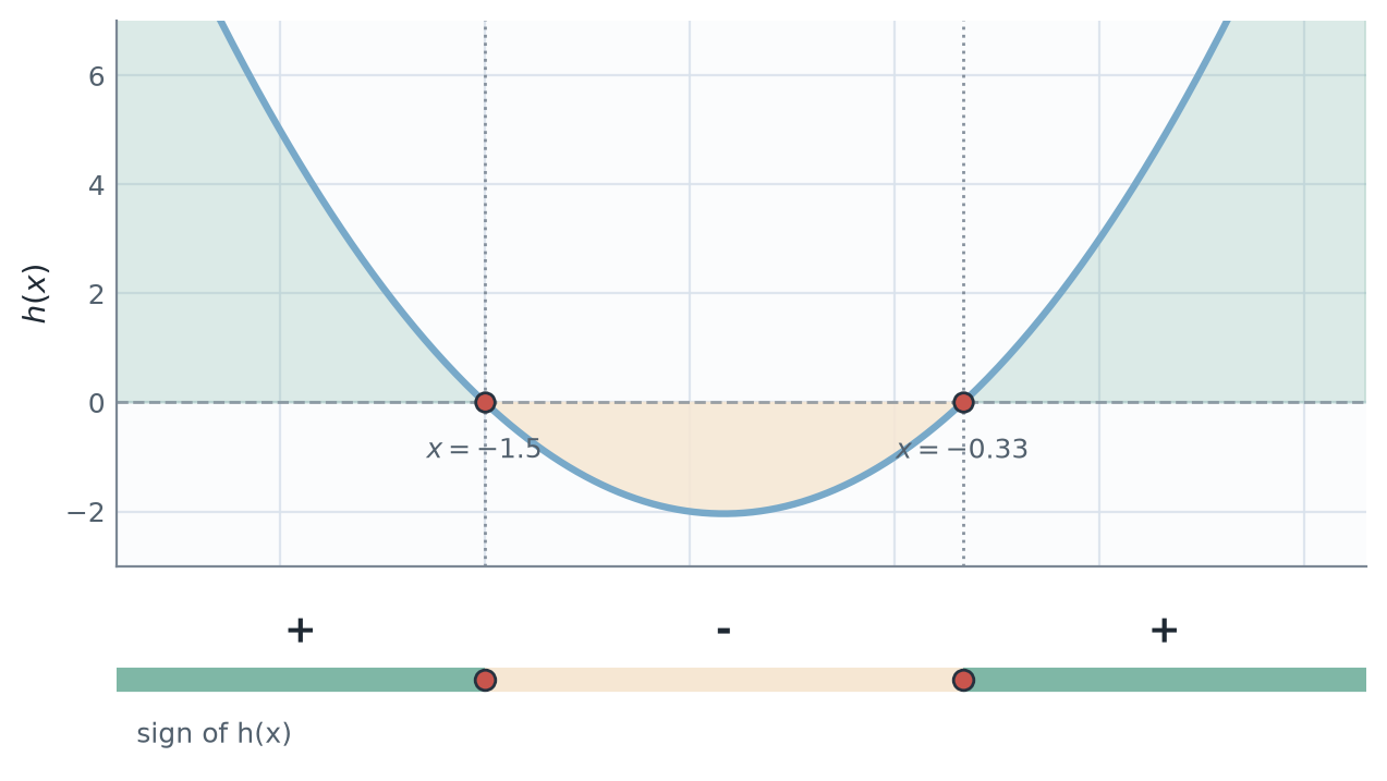
Graphically, this corresponds to whether the graph of the function lies above (positive) or below (negative) the -axis.
For a continuous function on an interval, the sign can change only at a root. In particular, polynomials are continuous, so their roots divide the real line into intervals on which the sign remains constant. When a domain has a gap, different domain components can have different signs without a root between them. For example, is continuous on each interval and , but it is undefined at and has opposite signs on the two components.
A polynomial need not change sign at every root. It crosses the -axis at a root of odd multiplicity, while it touches the axis and turns around at a root of even multiplicity.
For our quadratic function , we found earlier, that the roots are:
These roots divide the real line into three intervals:
By testing a single point in each interval (for instance, ), we find:
Table 7.1. Sign of on intervals determined by its roots.
| Interval | Test Value | Sign of | Behavior |
|---|---|---|---|
| is positive | |||
| is negative | |||
| is positive |
Solving Inequalities
Equations ask where two expressions are equal. Inequalities ask where one expression is less than, greater than, less than or equal to, or greater than or equal to another expression. The answer is often not a single number, but a set of numbers.
For example, solving
means finding all input values for which the graph of lies above the -axis. This connects inequalities directly to the sign analysis introduced above.
The solution set of an inequality is the set of all values that make the inequality true.
For one-variable inequalities, solution sets are often written using interval notation or set-builder notation.
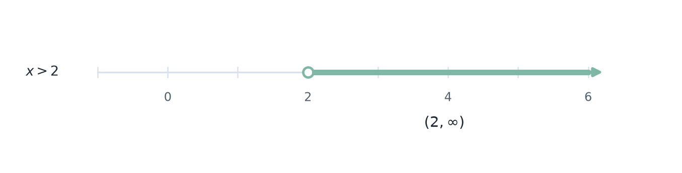
The inequality
has solution set
To solve a linear inequality:
- Simplify both sides.
- Collect the variable terms on one side and the constant terms on the other.
- If the coefficient of the variable is nonzero, divide by it. If it is negative, reverse the inequality sign.
- If the variable terms cancel, determine whether the remaining statement is always true or always false.
- Write the final solution set using interval or set-builder notation.
When multiplying or dividing both sides of an inequality by a negative number, the direction of the inequality must be reversed.
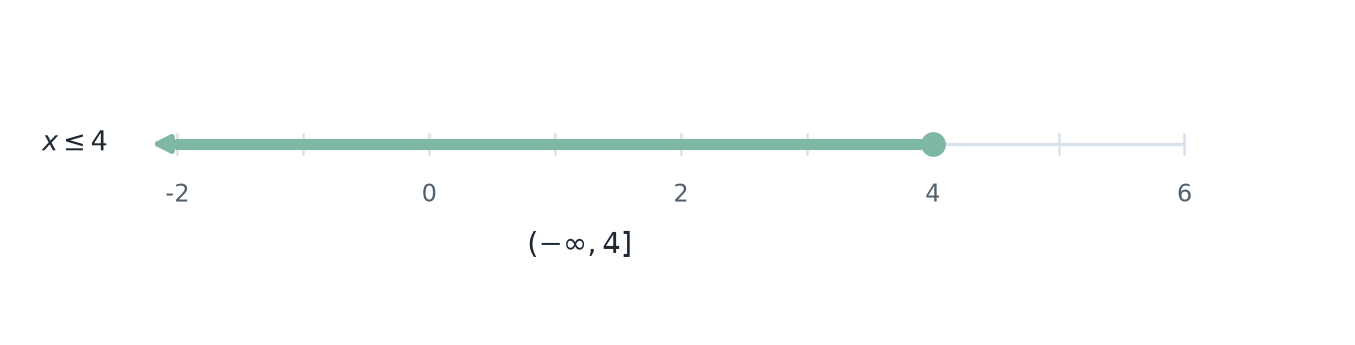
Solve
We isolate :
The solution set is
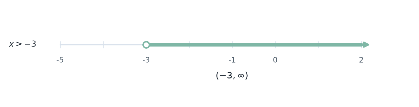
Solve
Dividing both sides by reverses the inequality sign:
The solution set is
Some inequalities combine two conditions. Logical symbols make the distinction between conditions and their solution sets precise. If and are inequality predicates, then requires both conditions, while requires at least one. The corresponding solution sets are combined using intersection and union, respectively.
A compound inequality is an inequality statement that combines two or more inequalities.
- A statement using and, written with , requires both inequalities to be true, so the solution set is an intersection.
- A statement using or, written with , requires at least one inequality to be true, so the solution set is a union.
For example, is shorthand for the conjunction
To solve a compound inequality:
- Separate the compound statement into its individual inequalities.
- Solve each inequality.
- Combine the individual solution sets using intersection for and or union for or.
- Write the final solution set using interval notation.
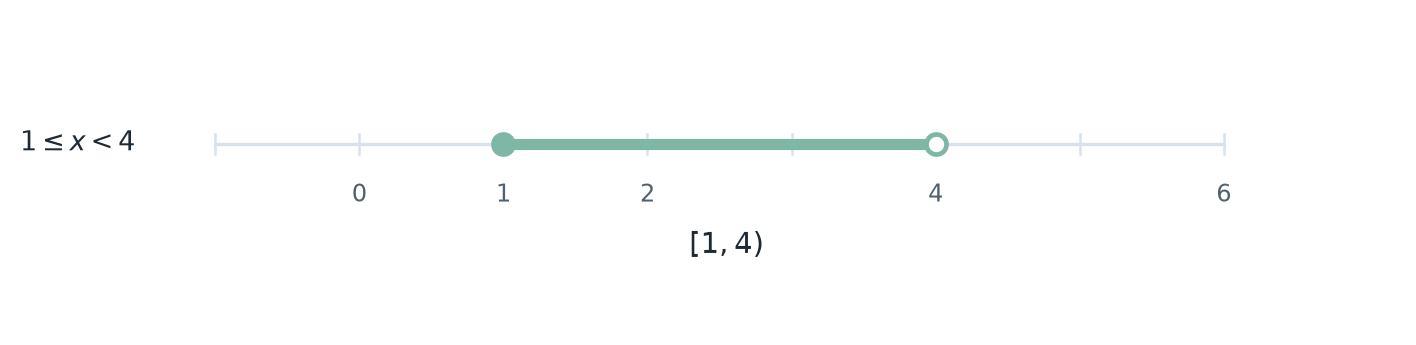
Solve
We isolate throughout the compound inequality:
The solution set is
The bracket at means that is included, while the parenthesis at means that is not included.
Solve
The connective means that a value only needs to satisfy one of the two inequalities. Therefore, the solution set is the union
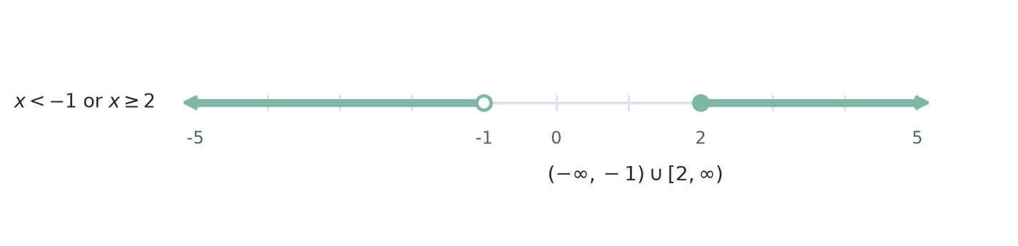
Polynomial inequalities can be solved by first finding the roots and then checking the sign of the expression on the intervals determined by those roots.
To solve a polynomial inequality such as or :
- Move all terms to one side so the inequality compares a function with .
- Find the roots of the function.
- Use the roots to divide the real line into intervals.
- Test one value in each interval to determine the sign of the function.
- Select the intervals on which the sign satisfies the inequality.
- Include roots for or , and exclude them for or .
- Write the final solution set using interval notation.
Solve
The roots are and . These split the real line into three intervals:
Testing one value from each interval gives:
Table 7.2. Sign test for .
| Interval | Test value | Sign of |
|---|---|---|
| Positive | ||
| Negative | ||
| Positive |
We need the expression to be greater than or equal to , so we choose the positive intervals and include the roots:
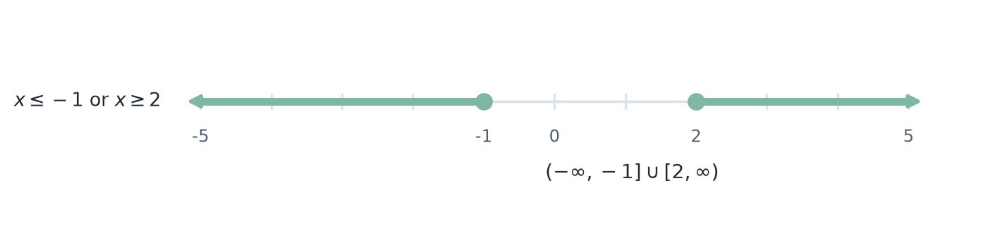
The union symbol appears naturally here because the solution consists of two separate intervals. This is one reason why the set operations from Chapter 2 are useful when solving inequalities.
Equation solving for exponential and logarithmic functions continues in Chapter 8, after inverse functions and logarithm rules have been introduced.