Chapter 15: Probability

Probability gives us a way to measure how likely it is that something will happen. We use probabilities when reasoning about uncertainty, making decisions, and interpreting information in areas such as weather forecasts, games, business decisions, insurance, and data science models.

In this chapter, we use two complementary viewpoints. Sometimes probabilities can be computed from a mathematical model of the possible outcomes. Other times, probabilities are estimated from repeated observations or collected data. Both viewpoints use the same basic language of experiments, outcomes, sample spaces, and events.

Probability Terminology

Before discussing how to find probabilities, we need a few basic terms.

Definitions: Probability Terminology

These terms describe the possible results of a random experiment and the collections of results we want to study.

Random experiment. A random experiment is an activity or operation with a result that cannot be predicted ahead of time.

Outcome. An outcome is any possible result from conducting an experiment.

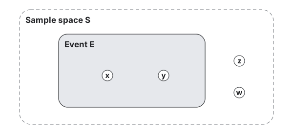
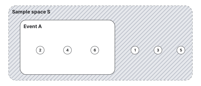
A dashed sample space S containing an event E. Outcomes x and y lie inside E, while outcomes z and w lie elsewhere in S. — Figure 15.1. The sample space $S$ contains all possible outcomes. The event $E \subseteq S$ contains the outcomes $x$ and $y$ , while $z$ and $w$ are outcomes in $S$ but not in $E$ .

Sample space. The sample space, usually denoted $S$ , is the set of all possible outcomes of an experiment.

Event. An event, denoted $E$ , is a subset of the sample space and describes a collection of outcomes.

Example: Rolling a Die

Consider an experiment of rolling a regular six-sided die. There are six possible outcomes, so the sample space is

$S = {1, 2, 3, 4, 5, 6} .$

Examples of events include:

Rolling a 2: $A = {2}$ .
Rolling an even number: $B = {2, 4, 6}$ .
Rolling a number greater than 4: $C = {5, 6}$ .

Example: Tossing Two Coins

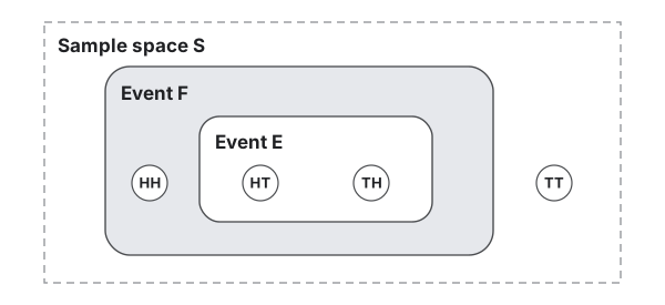
Two distinguishable coins, labeled 1 and 2, are tossed at the same time. In each outcome, the first letter records Coin 1 and the second records Coin 2. The sample space is

$S = {HH, H T, T H, TT} .$

If event $F$ is "getting at least one head," then

$F = {HH, H T, T H} .$

If event $E$ is "getting one head and one tail," then

$E = {H T, T H} .$

A dashed sample space S containing the nested events E and F. HT and TH lie in E, HH lies in F but outside E, and TT lies outside F. — Figure 15.2. The nested regions show $E \subset F \subset S$ : $H T$ and $T H$ belong to both events, $HH$ belongs only to $F$ , and $TT$ belongs to neither event.

Example: Coin and Die Outcomes

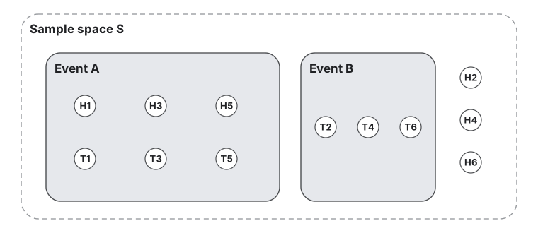
Gabe performs an experiment of flipping a coin and then rolling a regular six-sided die.

The sample space contains all possible coin-die outcomes:

$S = {H 1, H 2, H 3, H 4, H 5, H 6, T 1, T 2, T 3, T 4, T 5, T 6} .$

If event $A$ is "rolls an odd number," then

$A = {H 1, H 3, H 5, T 1, T 3, T 5} .$

If event $B$ is "gets tails and rolls an even number," then

$B = {T 2, T 4, T 6} .$

A dashed sample space S containing separate event regions A and B. The outcomes H2, H4, and H6 lie outside both events. — Figure 15.3. The separate regions show that events $A$ and $B$ are mutually exclusive, or disjoint, subsets of $S$ . The outcomes $H 2$ , $H 4$ , and $H 6$ lie outside both events.

Theoretical Probability

One way to learn about a probability is to repeat an experiment many times and record how often an event occurs. This is not always practical, and in some situations it is not necessary. For simple experiments such as rolling a fair die or drawing from a well-shuffled deck of cards, we can often compute probabilities directly from a mathematical model of the sample space.

The key assumption in this section is that all outcomes in the sample space are equally likely. This means that every individual outcome has the same chance of occurring. Under this assumption, finding the probability of an event becomes a counting problem: count the outcomes in the event and compare that number with the total number of outcomes in the sample space.

Definition: Probability

Probability is a numerical measure of the likelihood that an event will occur. If $E$ is an event, then $P (E)$ denotes the probability that event $E$ occurs.

Definition: Theoretical Probability

A theoretical probability is based on a mathematical model for the sample space.

$P$ can be viewed as a function: it takes an event $E \subseteq S$ as input and returns a number between $0$ and $1$ . The value $P (E)$ is the probability that event $E$ occurs.

Under the equally likely model, if $E$ is an event in a finite sample space $S$ , then

$P (E) = \frac{number of outcomes in event E}{number of outcomes in sample space S} = \frac{∣ E ∣}{∣ S ∣} .$

In this model, each single outcome $s \in S$ has probability

$P ({s}) = \frac{1}{∣ S ∣} .$

Example: Rolling a Six-Sided Die

Using the equally likely die model, start with the sample space and then count how many outcomes belong to each event.

Let

$S = {1, 2, 3, 4, 5, 6} .$

Define the events

$A = {2}, B = {2, 4, 6}, C = {5, 6} .$

Find the probability of each event:

Rolling a 2, represented by $A$ : $P (A) = \frac{1}{6} .$
Rolling an even number, represented by $B$ : $P (B) = \frac{3}{6} = \frac{1}{2} .$
Rolling a number greater than 4, represented by $C$ : $P (C) = \frac{2}{6} = \frac{1}{3} .$
Rolling a 7: $P (\emptyset) = \frac{0}{6} = 0.$
Rolling a number less than 7: $P (S) = \frac{6}{6} = 1.$

Note: When Outcomes Are Not Equally Likely

The counting formula

$P (E) = \frac{∣ E ∣}{∣ S ∣}$

only applies when all outcomes in the sample space are equally likely.

For a finite or countable discrete sample space whose outcome probabilities are known, the probability of an event is found by adding the probabilities of the outcomes in that event:

$P (E) = s \in E \sum P ({s}) .$

Example: A Loaded Die

Suppose a loaded six-sided die has sample space

$S = {1, 2, 3, 4, 5, 6},$

but the outcomes are not equally likely. For example, suppose

$P ({1}) = P ({2}) = P ({3}) = P ({4}) = P ({5}) = 0.15, P ({6}) = 0.25.$

These probabilities add to $1$ , so they define a valid probability model for the individual outcomes.

If $A$ is the event of rolling an even number, then

$A = {2, 4, 6} .$

Since the outcomes are not equally likely, we do not use $\frac{∣ A ∣}{∣ S ∣} = \frac{3}{6}$ . Instead,

$P (A) = P ({2}) + P ({4}) + P ({6}) = 0.15 + 0.15 + 0.25 = 0.55.$

The examples above motivate the following basic properties of valid probabilities.

Properties: Probability

Impossible event. An event that cannot occur has probability $0$ . In set notation, the impossible event is the empty set. If $E = \emptyset$ , then

$P (E) = P (\emptyset) = 0.$

Certain event. An event that must occur has probability $1$ . The sample space $S$ is the certain event. If $E = S$ , then

$P (E) = P (S) = 1.$

Partition of the sample space. If events $E_{1}, E_{2}, \dots, E_{k}$ are mutually exclusive and together cover the whole sample space, then

$P (E_{1}) + P (E_{2}) + \dots + P (E_{k}) = 1.$

Bounds. The probability of any event must be between $0$ and $1$ , inclusive:

$0 \leq P (E) \leq 1.$

Combining Events

The set operations introduced in Chapter 2 provide a compact way to describe events that occur together or separately.

Definitions: Unions and Intersections of Events

Let $E$ and $F$ be events in the same sample space.

Union. The event $E \cup F$ occurs when $E$ occurs, $F$ occurs, or both occur.

Intersection. The event $E \cap F$ occurs when both $E$ and $F$ occur.

Mutually exclusive events. Events $E$ and $F$ are mutually exclusive, or disjoint, if they cannot occur in the same trial. In set notation,

$E \cap F = \emptyset.$

When adding $P (E)$ and $P (F)$ , outcomes in $E \cap F$ have been counted twice. Subtracting their probability once gives the addition rule.

Rule: Addition Rule

For any two events $E$ and $F$ ,

$P (E \cup F) = P (E) + P (F) - P (E \cap F) .$

If $E$ and $F$ are mutually exclusive, then $P (E \cap F) = 0$ , so

$P (E \cup F) = P (E) + P (F) .$

Example: Union and Intersection

Roll a fair six-sided die. Let $A$ be the event of rolling an even number and let $B$ be the event of rolling a number greater than $3$ . Then

$A = {2, 4, 6}, B = {4, 5, 6}, A \cap B = {4, 6} .$

Therefore,

$P (A \cup B) = \frac{3}{6} + \frac{3}{6} - \frac{2}{6} = \frac{4}{6} = \frac{2}{3} .$

The result can be checked directly because $A \cup B = {2, 4, 5, 6}$ contains four of the six equally likely outcomes.

Conditional Probability and Independence

Sometimes additional information changes the sample space under consideration. Conditional probability describes this change.

Definition: Conditional Probability

If $P (F) > 0$ , the probability of $E$ given that $F$ has occurred is

$P (E ∣ F) = \frac{P ( E \cap F )}{P ( F )} .$

Rearranging this definition gives the multiplication rule

$P (E \cap F) = P (E ∣ F) P (F) .$

Example: Conditional Probability

One card is drawn from a well-shuffled standard deck. Let $E$ be the event that the card is an ace and $F$ the event that it is a spade. Given that the card is a spade, only the $13$ spades remain under consideration, and one of them is an ace. Thus,

$P (E ∣ F) = \frac{1}{13} .$

Definition: Independent Events

Events $E$ and $F$ are independent if knowing that one occurred does not change the probability of the other. Equivalently,

$P (E \cap F) = P (E) P (F) .$

If $P (F) > 0$ , this is equivalent to $P (E ∣ F) = P (E)$ .

Warning: Mutually Exclusive vs. Independent

Mutually exclusive events cannot occur together. Independent events do not affect each other's probabilities. If two events have positive probability and are mutually exclusive, then they are not independent because their intersection has probability $0$ .

Example: Independent Trials

Flip a fair coin and roll a fair six-sided die independently. Let $E$ be the event of getting heads and $F$ the event of rolling a $6$ . Then

$P (E \cap F) = P (E) P (F) = \frac{1}{2} \cdot \frac{1}{6} = \frac{1}{12} .$

A Minimal Counting Rule

Suppose an experiment is repeated $n$ times. We call the occurrence of an event of interest on any trial a success. If we want exactly $x$ successes, those successes can occur in different positions within the sequence. For instance, two successes in five trials could occur in the first two trials, the first and third trials, and so on.

To determine the probability of exactly $x$ successes, we must account for every possible arrangement of those successes among the $n$ trials. The binomial coefficient counts these arrangements.

Definition: Binomial Coefficient

The binomial coefficient

$(x n) = \frac{n !}{x ! ( n - x )!}$

counts the number of ways to choose $x$ positions from $n$ positions, where $n$ and $x$ are integers satisfying $n \geq 0$ and $0 \leq x \leq n$ . Here $n! = n (n - 1) \dots 2 \cdot 1$ and $0! = 1$ .

Example: Two Successes in Five Trials

Suppose five trials contain exactly two successes. Write $S$ for success and $F$ for failure. Each arrangement is determined by choosing which two of the five positions contain the successes. Therefore,

$(2 5) = \frac{5 !}{2 ! 3 !} = 10,$

so there are $10$ possible arrangements. For example, $SFSFF$ has successes in positions $1$ and $3$ .

Complements

Complements use the set-theoretic idea from Chapter 2: instead of counting outcomes in an event, we can sometimes count the outcomes not in it.

Definition: Complement

If $E$ is an event in sample space $S$ , then the complement of $E$ , denoted $E^{'}$ , is the set of all outcomes in $S$ that are not in $E$ :

$E^{'} = S ∖ E .$

The events $E$ and $E^{'}$ are mutually exclusive and together cover the entire sample space. Therefore,

$P (E) + P (E^{'}) = 1,$

$P (E^{'}) = 1 - P (E) .$

A dashed sample space S containing event E, with its complement shown by diagonal hatching outside E. — Figure 15.4. An event and its complement split the sample space $S$ into two disjoint parts whose probabilities add to one.

Example: Complement of an Event

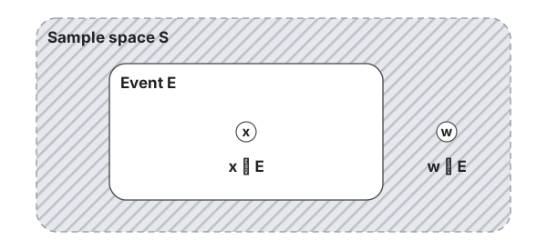
Roll a fair six-sided die and let

$A = {2, 4, 6}$

be the event of rolling an even number. Then the complement is the event of rolling an odd number:

$A^{'} = {1, 3, 5} .$

Since $P (A) = \frac{3}{6} = \frac{1}{2}$ ,

$P (A^{'}) = 1 - P (A) = 1 - \frac{1}{2} = \frac{1}{2} .$

A dashed die sample space S with the even outcomes inside event A and the odd outcomes in the hatched complement. — Figure 15.5. The even outcomes lie in $A$ ; the odd outcomes lie in the diagonally hatched complement $A^{'}$ . Together, the two regions cover the sample space $S$ .

Empirical Probability

Theoretical probability depends on a model. In many real situations, however, the model may be unknown, too complicated, or not based on equally likely outcomes. In those cases, we can estimate probabilities from data by repeating or observing the experiment and recording how often the event occurs.

Definitions: Theoretical and Empirical Probability

These two terms distinguish model-based probabilities from data-based estimates.

Theoretical probability. A theoretical probability is computed from a mathematical model.

Empirical probability. An empirical probability is an estimate based on collected data. After $n$ trials, if the event $E$ occurs $k$ times, its relative frequency is

$P (E) = \frac{k}{n} = \frac{number of times E occurs}{number of trials} .$

Note: Fractions, Decimals, Percentages, and Proportions

Probabilities are numbers between $0$ and $1$ . They can be written as fractions, decimals, or proportions on this scale.

To write the same quantity as a percentage, multiply the decimal by $100$ and add the percent sign. For example,

$\frac{1}{2} = 0.5, 0.5 \cdot 100 = 50,$

so $\frac{1}{2}$ is $50%$ when written as a percentage.

A relative frequency is an observed proportion: it tells us what fraction of the trials produced an event. It can also be reported as a percentage by multiplying the proportion by $100$ .

Example: Empirical Probability with Two Coins

Suppose two distinguishable fair coins are tossed independently and we are interested in the event

$E = {H T, T H},$

meaning exactly one head and one tail.

The theoretical probability is

$P (E) = \frac{∣ E ∣}{∣ S ∣} = \frac{2}{4} = \frac{1}{2} = 0.5.$

As a percentage, multiply by $100$ : $0.5 \cdot 100 = 50$ , so this is $50%$ .

If we perform the experiment $10$ times and observe $H T$ or $T H$ in $7$ of the trials, then the empirical probability is

$P (E) = \frac{7}{10} = 0.7.$

As a percentage, multiply by $100$ : $0.7 \cdot 100 = 70$ , so this is $70%$ .

The empirical probability differs from the theoretical probability because it is based on a small number of trials.

Example: Theoretical and Empirical Probability

Consider drawing one card at random from a well-shuffled standard 52-card deck and recording whether the card is a queen.

The theoretical probability of drawing a queen is

$\frac{4}{52} = \frac{1}{13} \approx 0.0769,$

which is about $0.0769 \cdot 100 = 7.69$ , so about $7.69%$ .

If the experiment is repeated $25$ times, with the card replaced each time, and a queen is drawn $3$ times, then the empirical probability is

$\frac{3}{25} = 0.12,$

which is $0.12 \cdot 100 = 12$ , so $12%$ .

The Law of Large Numbers

Empirical probabilities can vary substantially when the number of trials is small. As the number of trials increases, they tend to stabilize near the theoretical probability.

Law: The Law of Large Numbers

The Law of Large Numbers states that, over many independent repetitions of the same experiment, the empirical probability of an event tends to approach its theoretical probability.

For repeated independent tosses of two distinguishable fair coins, the event $E = {H T, T H}$ has theoretical probability $\frac{1}{2}$ . Suppose the experiment is repeated many times:

Table 15.1. Empirical probability of one head and one tail over repeated trials.

Number of Trials	Times $E$ Observed	Empirical Probability $P (E)$
10	7	$\frac{7}{10} = 70%$
20	13	$\frac{13}{20} = 65%$
30	17	$\frac{17}{30} \approx 56.7%$
40	22	$\frac{22}{40} = 55%$
50	26	$\frac{26}{50} = 52%$

Notice that the empirical probability begins to approach the theoretical probability $P (E) = \frac{1}{2}$ .

Running empirical probability of one head and one tail converging toward 0.5 over repeated two-coin tosses. — Figure 15.6. The running empirical probability for $E = {H T, T H}$ fluctuates but gradually stabilizes near the theoretical value $P (E) = 0.5$ .

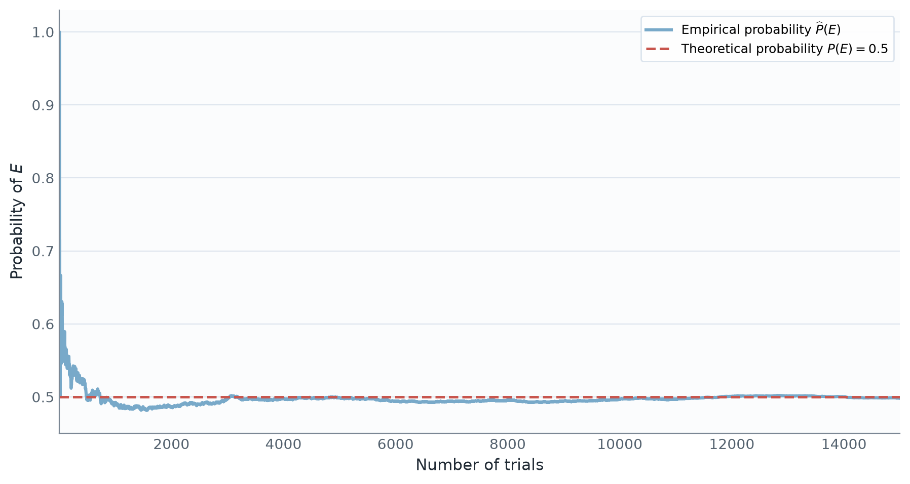
The table and figure show the main idea of the law: the empirical probability can fluctuate from trial to trial, but over many repetitions it tends to move closer to the theoretical probability. This approach is not necessarily monotone: after an additional trial, the estimate can temporarily move farther away before later moving closer again.

Keyboard shortcuts

Mathematics Brush-up for Data Science